Download Shortest Path in Graph Theory: Single Source, Negative Weights, Bellman-Ford and more Summaries Computer Networks in PDF only on Docsity!
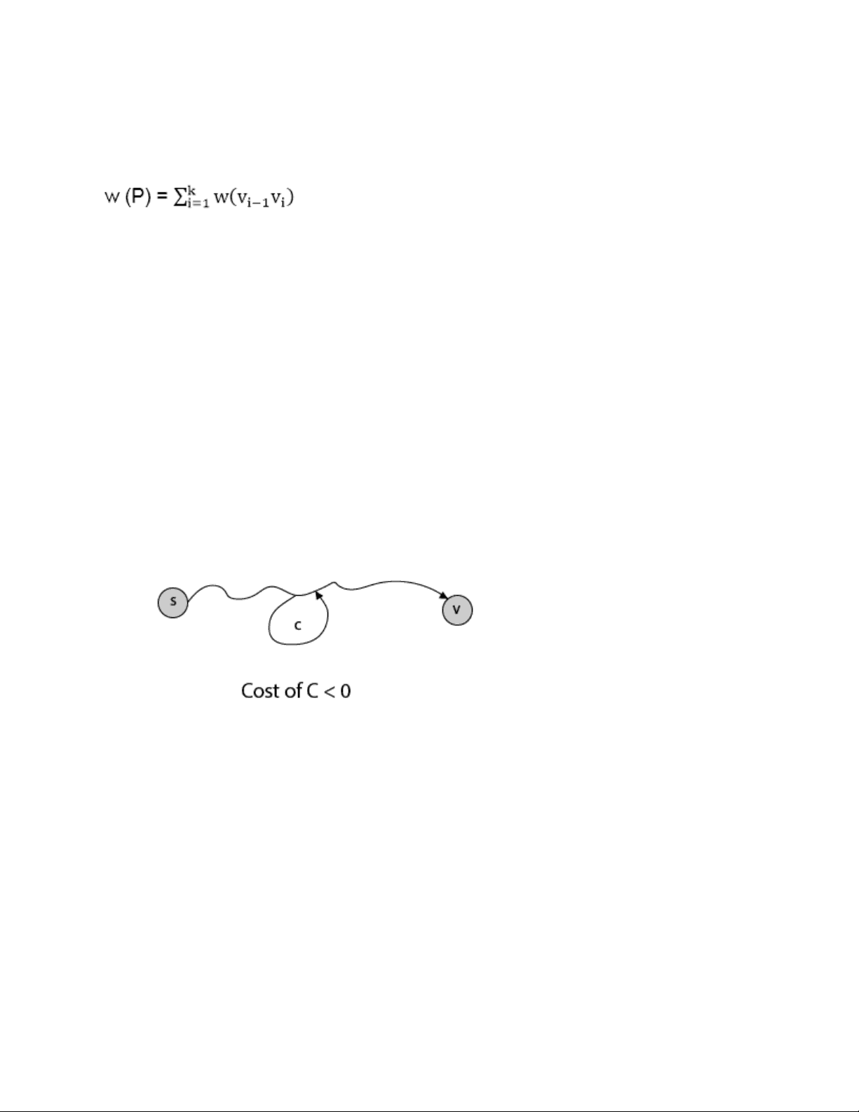
Single Source Shortest Paths Introduction: In a shortest- paths problem , we are given a weighted, directed graphs G = (V, E), with weight function w: E → R mapping edges to real-valued weights. The weight of path p = (v 0 ,v 1 ,..... vk) is the total of the weights of its constituent edges: We define the shortest - path weight from u to v by δ(u,v) = min (w (p): u→v), if there is a path from u to v, and δ(u,v)= ∞, otherwise. The shortest path from vertex s to vertex t is then defined as any path p with weight w (p) = δ(s,t). The breadth-first- search algorithm is the shortest path algorithm that works on unweighted graphs, that is, graphs in which each edge can be considered to have unit weight. In a Single Source Shortest Paths Problem , we are given a Graph G = (V, E), we want to find the shortest path from a given source vertex s ∈ V to every vertex v ∈ V. Variants: There are some variants of the shortest path problem.
- Single- destination shortest - paths problem: Find the shortest path to a given destination vertex t from every vertex v. By shift the direction of each edge in the graph, we can shorten this problem to a single - source problem.
- Single - pair shortest - path problem: Find the shortest path from u to v for given vertices u and v. If we determine the single - source problem with source vertex u, we clarify this problem also. Furthermore, no algorithms for this problem are known that run asymptotically faster than the best single - source algorithms in the worst case.
- All - pairs shortest - paths problem: Find the shortest path from u to v for every pair of vertices u and v. Running a single - source algorithm once from each vertex can clarify this problem; but it can generally be solved faster, and its structure is of interest in the own right. Shortest Path: Existence: If some path from s to v contains a negative cost cycle then, there does not exist the shortest path. Otherwise, there exists a shortest s - v that is simple. Negative Weight Edges It is a weighted graph in which the total weight of an edge is negative. If a graph has a negative edge, then it produces a chain. After executing the chain if the output is negative then it will give - ∞ weight and condition get discarded. If weight is less than negative and - ∞ then we can't have the shortest path in it. Briefly, if the output is - ve, then both condition get discarded.
- Not less than 0. And we cannot have the shortest Path.
Example:
- Beginning from s
- Adj [s] = [a, c, e]
- Weight from s to a is 3 Suppose we want to calculate a path from s→c. So We have 2 paths /weight
- s to c = 5 , s→c→d→c= 8
- But s→c is minimum
- So s→c = 5 Suppose we want to calculate a path from s→e. So we have two paths again
- s→e = 2 , s→e→f→e=- 1
- As - 1 < 0 ∴ Condition gets discarded. If we execute this chain, we will get - ∞. So we can't get the shortest pat h ∴ e = ∞. This figure illustrates the effects of negative weights and negative weight cycle on the shortest path weights. Because there is only one path from "s to a" (the path <s, a>), δ (s, a) = w (s, a) = 3. Furthermore, there is only one path from "s to b", so δ (s, b) = w (s, a) + w (a, b) = 3 + (-4) = - 1. There are infinite many path from "s to c" : <s, c> : <s, c, d, c>, <s, c, d, c, d, c> and so on. Because the cycle <c, d, c> has weight δ (c, d) = w (c, d) + w (d, c) = 6 + (-3) = 3, which is greater than 0, the shortest path from s to c is <s, c> with weight δ (s, c) = 5.
3. Upper-bound property: We always have d[v] ≥ δ(s, v) for all vertices v ∈ V, and once d[v] conclude the value δ(s, v), it never changes. 4. No-path property: If there is no path from s to v, then we regularly have d[v] = δ(s, v) = ∞. 5. Convergence property: If s->u->v is a shortest path in G for some u, v ∈ V, and if d[u] = δ(s, u) at any time prior to relaxing edge (u, v), then d[v] = δ(s, v) at all times thereafter. Relaxation The single - source shortest paths are based on a technique known as relaxation , a method that repeatedly decreases an upper bound on the actual shortest path weight of each vertex until the upper bound equivalent the shortest - path weight. For each vertex v ∈ V, we maintain an attribute d [v], which is an upper bound on the weight of the shortest path from source s to v. We call d [v] the shortest path estimate. INITIALIZE - SINGLE - SOURCE (G, s) 1. for each vertex v ∈ V [G] 2. do d [v] ← ∞ 3. π [v] ← NIL 4. d [s] ← 0 After initialization, π [v] = NIL for all v ∈ V, d [v] = 0 for v = s, and d [v] = ∞ for v ∈ V - {s}. The development of relaxing an edge (u, v) consists of testing whether we can improve the shortest path to v found so far by going through u and if so, updating d [v] and π [v]. A relaxation step may decrease the value of the shortest
- path estimate d [v] and updated v's predecessor field π [v]. Fig: Relaxing an edge (u, v) with weight w (u, v) = 2. The shortest-path estimate of each vertex appears within the vertex. (a) Because v. d > u. d + w (u, v) prior to relaxation, the value of v. d decreases
(b) Here, v. d < u. d + w (u, v) before relaxing the edge, and so the relaxation step leaves v. d unchanged. The subsequent code performs a relaxation step on edge (u, v) RELAX (u, v, w)
- If d [v] > d [u] + w (u, v)
- then d [v] ← d [u] + w (u, v)
- π [v] ← u Dijkstra's Algorithm It is a greedy algorithm that solves the single-source shortest path problem for a directed graph G = (V, E) with nonnegative edge weights, i.e., w (u, v) ≥ 0 for each edge (u, v) ∈ E. Dijkstra's Algorithm maintains a set S of vertices whose final shortest - path weights from the source s have already been determined. That's for all vertices v ∈ S; we have d [v] = δ (s, v). The algorithm repeatedly selects the vertex u ∈ V - S with the minimum shortest - path estimate, insert u into S and relaxes all edges leaving u. Because it always chooses the "lightest" or "closest" vertex in V - S to insert into set S, it is called as the greedy strategy. Dijkstra's Algorithm (G, w, s)
- INITIALIZE - SINGLE - SOURCE (G, s)
- S←∅
- Q←V [G]
- while Q ≠ ∅
- do u ← EXTRACT - MIN (Q)
- S ← S ∪ {u}
- for each vertex v ∈ Adj [u]
- do RELAX (u, v, w) Analysis: The running time of Dijkstra's algorithm on a graph with edges E and vertices V can be expressed as a function of |E| and |V| using the Big - O notation. The simplest implementation of the Dijkstra's algorithm stores vertices of set Q in an ordinary linked list or array, and operation Extract - Min (Q) is simply a linear search through all vertices in Q. In this case, the running time is O (|V^2 |+|E|=O(V^2 ). Example:
Step 3: Now find the adjacent of y that is t, x, z.
- Adj [y] → t, x, z [Here y is u and t, x, z are v] Case - (i) y →t d [v] > d [u] + w [u, v] d [t] > d [y] + w [y, t] 10 > 5 + 3 10 > 8 Then d [t] ← 8 π [t] ← y Case - (ii) y → x d [v] > d [u] + w [u, v] d [x] > d [y] + w [y, x] ∞ > 5 + 9 ∞ > 14 Then d [x] ← 14 π [x] ← 14 Case - (iii) y → z d [v] > d [u] + w [u, v] d [z] > d [y] + w [y, z] ∞ > 5 + 2 ∞ > 7 Then d [z] ← 7 π [z] ← y By comparing case (i), case (ii) and case (iii) Adj [y] → x = 14, t = 8, z = z is shortest z is assigned in 7 = [s, z] Step - 4 Now we will find adj [z] that are s, x
- Adj [z] → [x, s] [Here z is u and s and x are v] Case - (i) z → x d [v] > d [u] + w [u, v] d [x] > d [z] + w [z, x] 14 > 7 + 6 14 > 13
Then d [x] ← 13 π [x] ← z Case - (ii) z → s d [v] > d [u] + w [u, v] d [s] > d [z] + w [z, s] 0 > 7 + 7 0 > 14 ∴ This condition does not satisfy so it will be discarded. Now we have x = 13. Step 5: Now we will find Adj [t] Adj [t] → [x, y] [Here t is u and x and y are v] Case - (i) t → x d [v] > d [u] + w [u, v] d [x] > d [t] + w [t, x] 13 > 8 + 1 13 > 9 Then d [x] ← 9 π [x] ← t Case - (ii) t → y d [v] > d [u] + w [u, v] d [y] > d [t] + w [t, y] 5 > 10 ∴ This condition does not satisfy so it will be discarded. Thus we get all shortest path vertex as Weight from s to y is 5 Weight from s to z is 7 Weight from s to t is 8 Weight from s to x is 9 These are the shortest distance from the source's' in the given graph.
Solution: distk^ [u] = [min[distk-^1 [u],min[distk-^1 [i]+cost [i,u]]] as i ≠ u. dist^2 [2]=min[dist^1 [2],min[dist^1 [1]+cost[1,2],dist^1 [3]+cost[3,2],dist^1 [4]+cost[4,2],dist^1 [5]+cost[5,2]]] Min = [6, 0 + 6, 5 + (-2), ∞ + ∞ , ∞ +∞] = 3 dist^2 [3]=min[dist^1 [3],min[dist^1 [1]+cost[1,3],dist^1 [2]+cost[2,3],dist^1 [4]+cost[4,3],dist^1 [5]+cost[5,3]]] Min = [5, 0 +∞, 6 +∞, ∞ + ∞ , ∞ + ∞] = 5 dist^2 [4]=min[dist^1 [4],min[dist^1 [1]+cost[1,4],dist^1 [2]+cost[2,4],dist^1 [3]+cost[3,4],dist^1 [5]+cost[5,4]]] Min = [∞, 0 +∞, 6 + (-1), 5 + 4, ∞ +∞] = 5 dist^2 [5]=min[dist^1 [5],min[dist^1 [1]+cost[1,5],dist^1 [2]+cost[2,5],dist^1 [3]+cost[3,5],dist^1 [4]+cost[4,5]]] Min = [∞, 0 + ∞,6 + ∞,5 + 3, ∞ + 3] = 8 dist^3 [2]=min[dist^2 [2],min[dist^2 [1]+cost[1,2],dist^2 [3]+cost[3,2],dist^2 [4]+cost[4,2],dist^2 [5]+cost[5,2]]] Min = [3, 0 + 6, 5 + (-2), 5 + ∞ , 8 + ∞ ] = 3 dist^3 [3]=min[dist^2 [3],min[dist^2 [1]+cost[1,3],dist^2 [2]+cost[2,3],dist^2 [4]+cost[4,3],dist^2 [5]+cost[5,3]]] Min = [5, 0 + ∞, 3 + ∞, 5 + ∞,8 + ∞ ] = 5 dist^3 [4]=min[dist^2 [4],min[dist^2 [1]+cost[1,4],dist^2 [2]+cost[2,4],dist^2 [3]+cost[3,4],dist^2 [5]+cost[5,4]]] Min = [5, 0 + ∞, 3 + (-1), 5 + 4, 8 + ∞ ] = 2 dist^3 [5]=min[dist^2 [5],min[dist^2 [1]+cost[1,5],dist^2 [2]+cost[2,5],dist^2 [3]+cost[3,5],dist^2 [4]+cost[4,5]]] Min = [8, 0 + ∞, 3 + ∞, 5 + 3, 5 + 3] = 8
dist^4 [2]=min[dist^3 [2],min[dist^3 [1]+cost[1,2],dist^3 [3]+cost[3,2],dist^3 [4]+cost[4,2],dist^3 [5]+cost[5,2]]] Min = [3, 0 + 6, 5 + (-2), 2 + ∞, 8 + ∞ ] = dist^4 [3]=min[dist^3 [3],min[dist^3 [1]+cost[1,3],dist^3 [2]+cost[2,3],dist^3 [4]+cost[4,3],dist^3 [5]+cost[5,3]]] Min = 5, 0 + ∞, 3 + ∞, 2 + ∞, 8 + ∞ ] = dist^4 [4]=min[dist^3 [4],min[dist^3 [1]+cost[1,4],dist^3 [2]+cost[2,4],dist^3 [3]+cost[3,4],dist^3 [5]+cost[5,4]]] Min = [2, 0 + ∞, 3 + (-1), 5 + 4, 8 + ∞ ] = 2 dist^4 [5]=min[dist^3 [5],min[dist^3 [1]+cost[1,5],dist^3 [2]+cost[2,5],dist^3 [3]+cost[3,5],dist^3 [5]+cost[4,5]]] Min = [8, 0 +∞, 3 + ∞, 8, 5] = 5