Download electrical circuit of electrical engineering and more Essays (university) Electrical Circuit Analysis in PDF only on Docsity!
Electric Circuits Analysis 2 Year
2.4 RLC circuit:
In this section, we consider more complex circuits, which contain both an inductor and a capacitor.
The result is a second-order differential equation for any voltage or current of interest. Now we need
two initial conditions to solve each differential equation.
Such circuits occur routinely in a wide variety of applications, including oscillators and frequency
filters. They are also very useful in modelling a number of practical situations, such as automobile
suspension systems, temperature controllers, and even the response of an airplane to changes in
elevator and aileron positions.
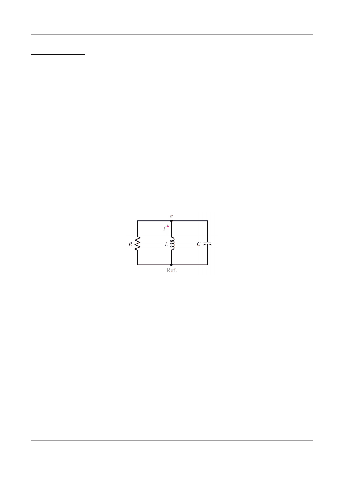
2.4.1 THE SOURCE-FREE PARALLEL CIRCUIT
When a physical capacitor is connected in parallel with an inductor and the capacitor has associated
with it a finite resistance, the resulting network can be shown to have an equivalent circuit model like
that shown in Fig. 2.28.
The presence of this resistance can be used to model energy loss in the capacitor; over time, all real
capacitors will eventually discharge, even if disconnected from a circuit. Energy losses in the
physical inductor can also be taken into account by adding an ideal resistor (in series with the ideal
inductor). For simplicity, however, we restrict our discussion to the case of an essentially ideal
inductor in parallel with a “leaky” capacitor.
Fig. 2.28: The source-free parallel RLC circuit.
In the following analysis, we will assume that energy may be stored initially in both the inductor and
the capacitor; in other words, nonzero initial values of both inductor current and capacitor voltage
may be present. With reference to the circuit of Fig. 2.28, we may then write the single nodal
equation
௩
ோ
ᇱ
௧
௧
బ
ௗ௩
ௗ௧
= 0 [1]
Note that the minus sign is a consequence of the assumed direction for i. We must solve Eq. [1]
subject to the initial conditions
i(
) = I
o
[2]
and
v(
) = V
o
[3]
When both sides of Eq. [1] are differentiated once with respect to time, the result is the linear
second-order homogeneous differential equation
ௗ
మ
௩
ௗ௧
మ
ଵ
ோ
ௗ௩
ௗ௧
ଵ
𝑣 = 0 [4]
whose solution v(t) is the desired natural response.
Electric Circuits Analysis 2 Year
We will assume a solution based on the exponential form. Thus, we assume
௦௧
[5]
Substituting Eq. [5] in Eq. [4], we obtain
ଶ
௦௧
ோ
௦௧
௦௧
௦௧
ଶ
ଵ
ோ
ଵ
ଶ
ଵ
ோ
ଵ
= 0 [6]
ଵ
ଵ
ଶோ
ଵ
ଶோ
ଶ
ଵ
[7]
ଶ
ଵ
ଶோ
ଵ
ଶோ
ଶ
ଵ
[8]
We thus have the general form of the natural response
ଵ
௦ భ
௧
ଶ
௦ మ
௧
[9]
where s 1
and s 2
are given by Eqs. [7] and [8]; A 1
and A 2
are two arbitrary constants which are to be
selected to satisfy the two specified initial conditions.
The form of the natural response as given in Eq. [9] offers little insight into the nature of the curve
we might obtain if v(t) were plotted as a function of time.
Since the exponents, s 1
t and s 2
t must be dimensionless, s 1
and s 2
must have the unit of some
dimensionless quantity “per second”. From Eqs. [7] and [8] we therefore see that the units of 1/2RC
and 1/√LC must also be s
(i.e., seconds
). Units of this type are called frequencies.
Let us define a new term, ω 0
(resonant frequency):
w
ଵ
√
[10]
On the other hand, we will call 1/2RC the neper frequency, or the exponential damping coefficient,
and represent it by the symbol α (alpha):
α =
ଵ
ଶୖେ
[11]
This latter descriptive expression is used because α is a measure of how rapidly the natural response
decays or damps out to its steady, final value (usually zero). Finally, s, s1, and s2, which are
quantities that will form the basis for some of our later work, are called complex frequencies.
Let us collect these results. The natural response of the parallel RLC circuit is
ଵ
௦
భ
௧
ଶ
௦
మ
௧
[9]
Where
ଵ
ଶ
ଶ
[12]
ଶ
ଶ
ଶ
[13]
We note two basic scenarios possible with Eqs. [12] and [13] depending on the relative sizes of α and
ω 0
(dictated by the values of R, L, and C). If α > ω 0 , s 1
and s 2
will both be real numbers, leading to
what is referred to as an overdamped response. In the opposite case, where α < ω 0
, both s 1
and s 2
will
have nonzero imaginary components, leading to what is known as an underdamped response. Both of
these situations are considered separately in the following sections, along with the special case of α =
ω 0
, which leads to what is called a critically damped response.
Electric Circuits Analysis 2 Year
We can obtain a second equation relating A 1
and A 2
by taking the derivative of v(t) with respect to
time in Eq. [14], determining the initial value of this derivative through the use of the remaining
initial condition i (0) = 10, and equating the results. So, taking the derivative of both sides of Eq.
[14],
ଵ
ି ௧
ଶ
ି ௧
and evaluating the derivative at t = 0,
௧ୀ
ଵ
ଶ
i C
= Cdv/dt
Kirchhoff’s current law must hold at any instant in time, as it is based on conservation of electrons.
Thus, we may write
−i C
(0) + i (0) + i R
Substituting our expression for capacitor current and dividing by C,
dv/dt| t=
= i C
(0)/C = (i (0) + i R
(0))/C = i (0)/C = 420 V/s
since zero initial voltage across the resistor requires zero initial current through it. We thus have our
second equation,
420 = −A
1
− 6A
2
[16]
and simultaneous solution of Eqs. [15] and [16] provides the two amplitudes A 1
= 84 and A 2
Therefore, the final numerical solution for the natural response of this circuit is
v(t) = 84(e
−t
− e
−6t
) V [17]
Example 2.9: Find an expression for vC(t) valid for t > 0 in the circuit of Fig. 2.30a.
Fig. 2.
Solution:
After the switch is thrown, the capacitor is left in parallel with a 200 Ω resistor and a 5 mH inductor
(Fig. 2.30b). Thus,
α = 1/2RC = 125,000 s
−
ω 0
= 1/√(LC) = 100,000 rad/s
s 1
= −α + √(α
2
2
) = −50,000 s
−
s 2
= −α − √(α
2
2
) = −200,000 s
−
Since α > ω 0
, the circuit is overdamped and so we expect a capacitor voltage of the form
ଵ
௦ భ
௧
ଶ
௦ మ
௧
Electric Circuits Analysis 2 Year
From Fig. 2.31a, in which the inductor has been replaced with a short circuit and the capacitor with
an open circuit, we see that
i L
) = − 150/(200 + 300) = −300 mA
and
v C
) = 150*200/(200 + 300) = 60 V
Fig. 2.
In Fig. 2.31b, we draw the circuit at t = 0
, representing the inductor current and capacitor voltage by
ideal sources for simplicity. Since neither can change in zero time, we know that v C
) = 60 V.
We have an equation for the capacitor voltage:
v C
(t) = A 1
e
−50,000t
+ A
2
e
−200,000t
We now know v C
(0) = 60 V, but a third equation is still required. Differentiating our capacitor
voltage equation, we find
dv C
/dt = −50,000A 1
e
−50,000t
− 200,000A
2
e
−200,000t
which can be related to the capacitor current as i C
= C(dv C
/dt).
Returning to Fig. 1.31b, KCL yields
i C
) = −i L
) − i R
) = 0.3 − [v C
)/200] = 0
Application of our first initial condition yields v C
(0) = A
1
+ A
2
= 60 and application of our second
initial condition yields
i C
(0) = −20 × 10
−
(50,000A
1
+ 200,000A
2
Solving, A 1
= 80 V and A 2
= −20 V, so that
v C
(t) = 80e
−50,000t
− 20e
−200,000t
V, t > 0
At the very least, we can check our solution at t = 0, verifying that v C
(0) = 60 V. Differentiating and
multiplying by 20 × 10
−
, we can also verify that i C
(0) = 0. Also, since we have a source-free circuit
for t > 0, we expect that v C
(t) must eventually decay to zero as t approaches ∞, which our solution
does.
Electric Circuits Analysis 2 Year
Example 2.10: For t > 0, the capacitor current of a certain source-free parallel RLC circuit is given
by i C
(t) = 2e
−2t
− 4e
−t
A. Sketch the current in the range 0 < t < 5 s, and determine the settling time.
Solution:
We first sketch the two terms as shown in Fig. 2.34, then subtract them to find i C
(t). The maximum
value is clearly |−2| = 2 A. We therefore need to find the time at which |i C
| has decreased to 20 mA,
or
2e
−2ts
− 4e
−ts
= −0.02 [1]
Fig. 2.
This equation can be solved using an iterative solver routine on a scientific calculator, which returns
the solution ts = 5.296 s. If such an option is not available, however, we can approximate Eq. [1] for t
≥ ts as
−4e
−ts
= −0.02 [2]
Solving, t s
= −ln(0.02/4) = 5.298 s
which is reasonably close (better than 0.1% accuracy) to the exact solution.
H.W.: (a) Sketch the voltage v R
(t) = 2e
−t
− 4e
−3t
V in the range 0 < t < 5 s. (b) Estimate the settling
time. (c) Calculate the maximum positive value and the time at which it occurs.
2.4.2 CRITICAL DAMPING
Now let us adjust the element values until α and ω 0
are equal. This is a very special case which is
termed critical damping.
Critical damping is achieved when
ଶ
ଶ
ଶ
ൡ Critical damping
Electric Circuits Analysis 2 Year
We will select R, increasing its value until critical damping is obtained, and thus leave ω
unchanged. The necessary value of R is 7√6/2 Ω; L is still 7 H, and C remains 1/42 F. We thus find
α = ω 0
= √6 s
−
s 1
= s 2
= −√6 s
−
and recall the initial conditions that were specified, v(0) = 0 and i(0) =10 A.
The differential equation of RLC parallel circuit is
ௗ
మ
௩
ௗ௧
మ
ଵ
ோ
ௗ௩
ௗ௧
ଵ
𝑣 = 0 [1]
When α = ω0, the differential equation, Eq. [1], becomes
ௗ
మ
௩
ௗ௧
మ
ௗ௩
ௗ௧
ଶ
The solution of this equation is not a tremendously difficult process, but we will avoid developing it
here, since the equation is a standard type found in the usual differential-equation texts. The solution
is
v = e
−αt
(A
1
t + A 2
) [2]
Let us now complete our numerical example. After we substitute the known value of α in Eq. [2],
obtaining
v = A 1
te
−√6t
+ A
2
e
−√6t
we establish the values of A 1
and A 2
by first imposing the initial condition on v(t) itself, v(0) = 0.
Thus, A2 = 0. The second initial condition must be applied to the derivative dv/dt just as in the
overdamped case. We therefore differentiate, remembering that A2 = 0:
dv/dt = A 1
t (−√6)e
−√6t
+ A
1
e
−√6t
evaluate at t = 0:
dv/dt | t=
= A
1
and express the derivative in terms of the initial capacitor current:
dv/dt | t=
= i C
(0)/C = (i R
(0)/C) + (i(0)/C)
A
1
= 420 V
The response is, therefore,
v(t) = 420te
−2.45t
V
Graphical Representation of the Critically Damped Response
and once again we have a response that begins and ends at zero and has positive values at all other
times. A maximum value v m
again occurs at time tm; for our example,
tm = 0.408 s and vm = 63.1 V
This maximum is larger than that obtained in the overdamped case, and is a result of the smaller
losses that occur in the larger resistor; the time of the maximum response is slightly later than it was
with overdamping. The settling time may also be determined by solving
v m
/100 = 420tse
−2.45ts
for ts (by trial-and-error methods or a calculator’s SOLVE routine):
ts = 3.12 s
Electric Circuits Analysis 2 Year
H.W.: (a) Choose R 1
in the circuit of Fig. 2.37 so that the response after t = 0 will be critically
damped. (b) Now select R 2
to obtain v(0) = 100 V. (c) Find v(t) at t = 1 ms.
Fig. 2.37.
2.4.3 THE UNDERDAMPED PARALLEL RLC CIRCUIT
The form of the underdamped response
ଵ
௦ భ
௧
ଶ
௦ మ
௧
where
ଵ,ଶ
ଵ
ଶோ
ଵ
ଶோ
ଶ
ଵ
and then let
ටα
ଶ
− w
ଶ
= √−1ටw
ଶ
− α
ଶ
= 𝑗ටw
ଶ
− α
ଶ
We now take the new radical, which is real for the underdamped case, and call it ω d
, the natural
resonant frequency:
ௗ
= ඥw
ଶ
− α
ଶ
The response may now be written as
ି ఈ௧
ଵ
௪
௧
ଶ
ି ௪
௧
൯ [1]
or, in the longer but equivalent form,
ି ఈ௧
ଵ
ଶ
௪
௧
ି ௪
௧
ଵ
ଶ
௪
௧
ି ௪
௧
ି ఈ௧
ଵ
ଶ
ௗ
ଵ
ଶ
ௗ
and the multiplying factors may be assigned new symbols:
ି ఈ௧
ଵ
ௗ
ଶ
ௗ
𝑡)} [2]
We return to our simple parallel RLC circuit with R = 6 Ω,
C = 1/42 F, and L = 7 H, but now increase the resistance
further to 10.5 Ω.
Thus,
ଵ
ଶோ
= 2 s
−
ି ଵ
Electric Circuits Analysis 2 Year
and
ௗ
w
ଶ
− α
ଶ
except for the evaluation of the arbitrary constants, the response is now known:
ି ଶ௧
ଵ
ଶ
The determination of the two constants proceeds as before. If we still assume that v(0) = 0 and i(0) =
10, then B 1
must be zero. Hence
ି ଶ௧
ଶ
The derivative is
ି ଶ௧
ଶ
ି ଶ௧
ଶ
and at t = 0 it becomes
௧ୀ
ଶ
where i C
is defined in figure. Therefore,
ି ଶ௧
Graphical Representation of the Underdamped Response
Returning to our specific numerical problem, differentiation locates the first maximum of v(t),
v m
= 71.8 V at t m
= 0.435 s
The succeeding minimum,
v m
= −0.845 V at t m
= 2.66 s
and so on. The response curve is shown in Fig. 2.38.
Fig. 2.
Electric Circuits Analysis 2 Year
Fig. 2.
H.W.: The switch in the circuit of Fig. 2.41 has been in the left position for a long time; it is moved to
the right at t = 0. Find (a) dv/dt at t = 0
; (b) v at t = 1 ms; (c) t 0
, the first value of t greater than
zero at which v = 0.
Fig. 2.
Electric Circuits Analysis 2 Year
2.4.4 THE SOURCE-FREE SERIES RLC CIRCUIT
Figure 2.42 shows the series circuit. The fundamental integrodifferential equation is
Fig. 2.42.
௧
௧ బ
The respective second-order equations obtained by differentiating these two equations with respect to
time are also duals:
ௗ
మ
ௗ௧
మ
ௗ
ௗ௧
ଵ
𝑖 = 0 [1]
In terms of the circuit shown in Fig. 2.42, the overdamped response is
ଵ
௦ భ
௧
ଵ
௦ భ
௧
where
ଵ,ଶ
ଶ
ଶ
ଶ
and thus
The form of the critically damped response is
ି ఈ௧
ଵ
ଶ
and the underdamped response may be written
ି ఈ௧
ଵ
ௗ
ଶ
ௗ
Where 𝜔
ௗ
ଶ
ଶ
Electric Circuits Analysis 2 Year
A good sketch may be made by first drawing in the two portions of the exponential envelope, 2e
−1000t
and −2e
−1000t
mA, as shown by the broken lines in Fig. 2.44. The location of the quarter-cycle points
of the sinusoidal wave at 20,000t = 0, π/2, π, etc., or t = 0.07854k ms, k = 0, 1, 2,.. ., by light marks
on the time axis then permits the oscillatory curve to be sketched in quickly.
Fig. 2.44.
H.W.: With reference to the circuit shown in Fig. 2.45, find (a) α; (b) ω 0
; (c) i(
); (d) di/dt| t=0+
; (e)
i (12 ms).
Fig. 2.45.
Example 2.14: Find an expression for v C
(t) in the circuit of Fig. 2.46a, valid for t > 0.
Fig. 2.46.
Electric Circuits Analysis 2 Year
Solution:
As we are interested only in v C
(t), it is perfectly acceptable to begin by finding the Thévenin
equivalent resistance connected in series with the inductor and capacitor at t = 0
. We do this by
connecting a 1 A source as shown in Fig. 2.46b, from which we deduce that
v test
= 11i − 3i = 8i = 8(1) = 8 V
Thus, Req =8 Ω, so α = R/2L =0.8 s
−
and 𝜔
ଵ
√
= 10 rad/s, meaning that we expect an
underdamped response with ω d
= 9.968 rad/s and the form
v C
(t) = e
−0.8t
(B
1
cos 9.968t + B 2
sin 9.968t) [1]
In considering the circuit at t = 0
−
, we note that i L
−
) = 0 due to the presence of the capacitor. By
Ohm’s law, i (
−
) = 5 A, so
v C
) = v C
−
) = 10 − 3i = 10 − 15 = −5 V
This last condition substituted into Eq. [1] yields B 1
= −5 V. Taking the derivative of Eq. [1] and
evaluating at t = 0 yield
dv C
/dt| t=
= −0.8B
1
+ 9.968B
2
= 4 + 9.968B
2
[2]
We see from Fig. 2.46a that
i = −Cdv C
/dt
Thus, making use of the fact that i (
) = i L
−
) = 0 in Eq. [2] yields
B
2
= −0.4013 V, and we may write
v C
(t) = −e
−0.8t
(5 cos 9.968t + 0.4013 sin 9.968t) V t > 0
H.W.: Find an expression for i L
(t) in the circuit of Fig. 2.47, valid for t > 0, if v C
−
) = 10 V and
i L
−
) = 0. Note that although it is not helpful to apply Thévenin techniques in this instance, the
action of the dependent source links v C
and i L
such that a first-order linear differential
equation results.
Fig. 2.47.
Electric Circuits Analysis 2 Year
- t = 0
During the interval from t = 0
−
to t = 0
, the left-hand current source becomes active and
many of the voltage and current values at t = 0
−
will change abruptly. The corresponding circuit is
shown in Fig. 2.48c. However, we should begin by focusing our attention on those quantities which
cannot change, namely, the inductor current and the capacitor voltage. Both of these must remain
constant during the switching interval. Thus,
i L
) = 5 A and v C
) = 150 V
Since two currents are now known at the left node, we next obtain
i R
) = −1 A and v R
) = −30 V
so that
i C
) = 4 A and v L
) = 120 V
and we have our six initial values at t = 0
−
and six more at t = 0
Among these last six values, only the capacitor voltage and the inductor current are unchanged from
the t = 0
−
values.
H.W.: Let i s
= 10u(−t) − 20u(t) A in Fig. 2.49. Find (a) i L
−
) (b) v C
); (c) v R
); (d) i L
(∞); (e)
i L
(0.1 ms).
Fig. 2.49.
Example 2.16: Complete the determination of the initial conditions in the circuit of Fig. 2.51, by
finding values at t = 0
for the first derivatives of the three voltage and three current variables
defined on the circuit diagram.
Fig. 2.51.
Solution:
We begin with the two energy storage elements. For the inductor,
and, specifically,
ା
௧ୀ
శ
Electric Circuits Analysis 2 Year
Thus,
௧ୀ
శ
ା
Similarly,
௧ୀ
శ
ା
The other four derivatives may be determined by realizing that KCL and KVL are both satisfied by
the derivatives also. For example, at the left-hand node in Fig. 2.51,
4 − i L
− i R
= 0 t > 0
and thus,
0 – di L
/dt− di R
/dt = 0 t > 0
and therefore,
ோ
௧ୀ
శ
The three remaining initial values of the derivatives are found to be
ோ
௧ୀ
శ
௧ୀ
శ
and
௧ୀ
శ