Download Element Nodal Displacement - Advanced Mechanics of Solids - Lecture Notes and more Study notes Applied Solid Mechanics in PDF only on Docsity!
Finite element method (continued)
Summary of essential concepts:
FEM analysis begins with calculations on the element level.
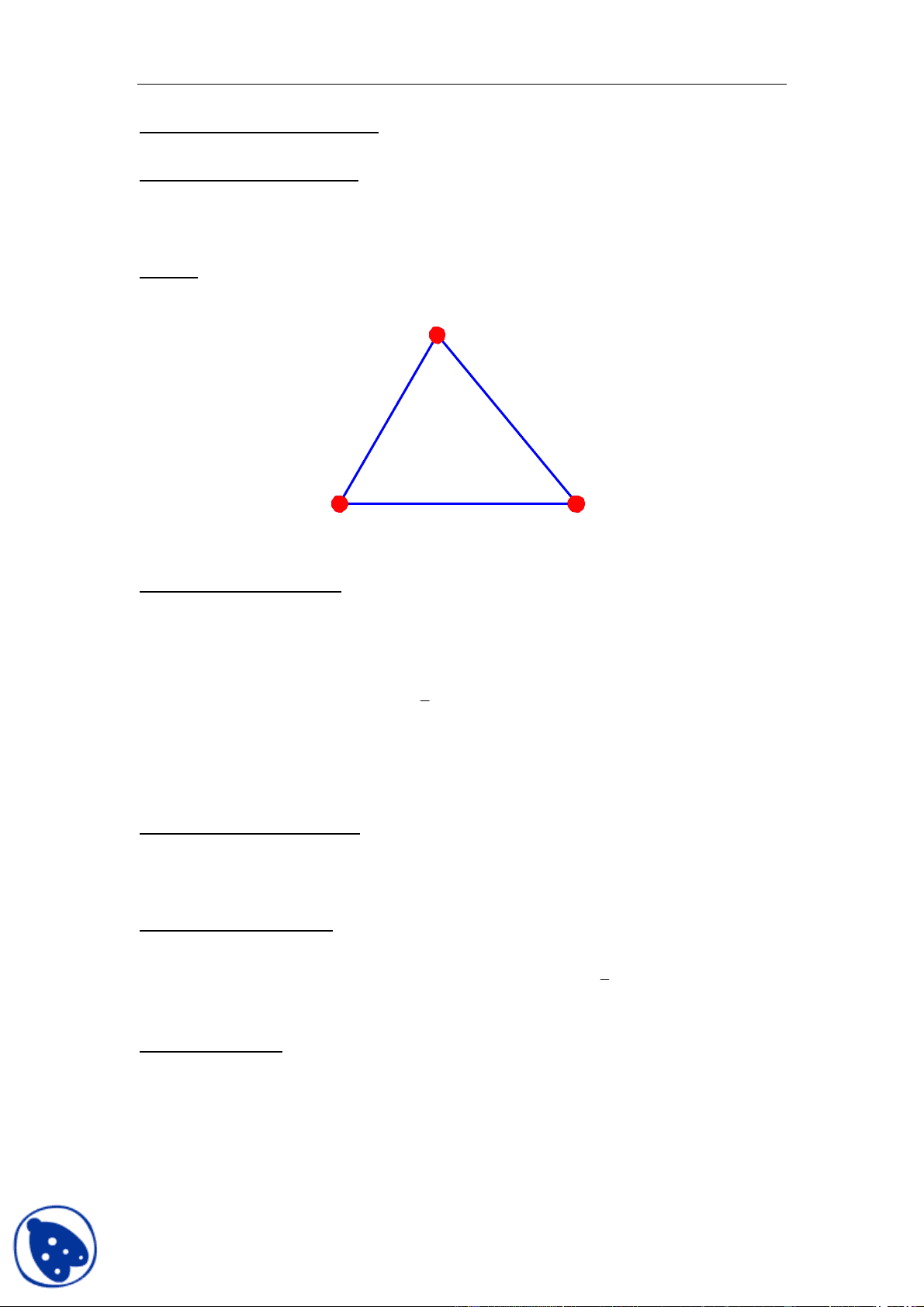
Element
Element nodal displacement:
3
2
3
1
2
2
2
1
1
2
1
1
u
u
u
u
u
u
u (^) el
Element interpolation function:
1
N x , x , ( 1 2 )
2
N x , x , ( 1 2 )
3 N x , x
Element displacement field:
u el N N N
N N N
u
u ⎥ ⎦
1 2 3
1 2 3
2
1
0 0 0
Element strain field:
1
uel Bu el
x
N
x
N
x
N
x
N
x
N
x
N
x
N
x
N
x
N
x
N
x
N
x
N
=
⎥
⎥
⎥
⎥
⎥
⎥
⎥
⎦
⎤
⎢
⎢
⎢
⎢
⎢
⎢
⎢
⎣
⎡
∂
∂
∂
∂
∂
∂
∂
∂
∂
∂
∂
∂
∂
∂
∂
∂
∂
∂
∂
∂
∂
∂
∂
∂
=
⎥
⎥
⎥
⎦
⎤
⎢
⎢
⎢
⎣
⎡
=
1
3
2
3
1
2
2
2
1
1
2
1
2
3
2
2
2
1
1
3
1
2
1
1
12
22
11
0 0 0
0 0 0
2 ε
ε
ε
ε
Element stress field:
D DBu el
E = =
⎥
⎥
⎥
⎦
⎤
⎢
⎢
⎢
⎣
⎡
⎥
⎥
⎥
⎥
⎦
⎤
⎢
⎢
⎢
⎢
⎣
⎡
− −
=
⎥
⎥
⎥
⎦
⎤
⎢
⎢
⎢
⎣
⎡
= ε
ε
ε
ε
ν
ν
ν
ν σ
σ
σ
σ
12
22
11
2
12
22
11
2 2
1 0 0
1 0
1 0
1
Element strain energy:
el el
T U (^) el (^) V ij ij V uelK u el (^) 2
1 d 2
1 = (^) ∫ σε =
K A B D B
T el = el
Element nodal force:
V f^ i^ ui V A tiui S Felu^ el el el
∫ ∫
d d
After the element quantities are calculated, the next step is to assemble the global stiffness matrix.
Global strain energy:
U U u K u u K u
T
elements
el el
T el elements
el 2
1
2
1
61
3
2
3
1
2
2
2
1
1
2
1
1
×
u
u
u
u
u
u
u (^) el Æ
( )
( )
( )
( )
( )
( )
2 1
3 2
3 1
2 2
2 1
1 2
1 1
×
n
u
u
u
u
u
u
u
M
( K el ) 6 × 6 Æ K 2 n × 2 n
Element connectivity
( # 1 ,# 2 ,# 3 ) ⇒( a , b , c )
α^ ( 1 , 2 , 3 , 4 , 5 , 6 )^ ⇒ z α(^2 a − 1 , 2 a , 2 b − 1 , 2 b , 2 c − 1 , 2 c )
2
( )
( )
( )
( )
( )
( )
( )
( )
( )
( )
( ) 2 2 , (^231)
1 2 1 , 2
42
2 2
32
2 1
12
1 1
2
1
2 2
2 1
1 2
1 1
2 , 1 2 , 3 2 , 2
31 33 3 , 2
11 13 1 , 2
×
− ⎥
n n
n
n
n
n
n
n n n n
n
n
F K
F K
F K
F K
F K
u
u
u
u
u
u
K K K
K K K
K K K
M^ M
L L L
M M M M M M M
M M M M M M M
M M M M M M
L L L
L L
L L L
The modified K then remains symmetric, as shown above.
Post-processing
Extract nodal displacement using element connectivity: u ⇒ uel
ε= Bu el
σ= DBu el
Isoparametric elements:
The actual nodal coordinates can be mapped to a normalized domain ξ ⊂ [− 1 , 1 ], which is
particularly convenient because displacements and positions for different elements can be
interpolated using the same shape functions.
1 # 2
x
− 1 0 1
ξ
1 1 # 2 2
u x = u N + u N
1 1 # 2 2
x = x N + x N
1 1 ,^1
N ξ , ( )
2 0 ,^1
N ξ
Interpolation functions:
N = , ( )
N =
4
2D linear triangular element:
a b
c
ξ 1
ξ 2
3 1 2
2 1 2
1
u u N ξ ,ξ u N ξ,ξ u N ξ, ξ
v v a v b v c = + +
3 1 2
2 1 2
1
x x N ξ ,ξ x N ξ,ξ x N ξ, ξ
v v a v b v c = + +
Interpolation functions:
1
N ξ = ξ, ( ) 2
2
N ξ = ξ , ( ) 12
3
N ξ = 1 −ξ − ξ
2D quadratic triangular element:
ξ 1
3
Interpolation functions:
1
N = 2 ξ − 1 ξ
2
N = 2 ξ − 1 ξ
3
N = 21 −ξ −ξ − 1 1 −ξ − ξ
1 2
4
N = 4 ξ ξ
2 (^12 )
5
N = 4 ξ 1 −ξ − ξ
5
Interpolation functions:
1 1 1 1 8
N = −ξ −ξ − ξ ), ( 1 )( 2 )( 3
2 1 1 1 8
N = +ξ −ξ − ξ)
3 1 1 1 8
N = +ξ +ξ − ξ), ( 1 )( 2 )( 3
4 1 1 1 8
N = −ξ +ξ − ξ )
5 1 1 1 8
N = −ξ −ξ + ξ), ( 1 )( 2 )( 3
6 1 1 1 8
N = +ξ −ξ + ξ )
7 1 1 1 8
N = +ξ +ξ + ξ ) , ( 1 )( 2 )( 3
8 1 1 1 8
N = −ξ +ξ + ξ)
Element stiffness matrix:
1 2 3
1
1
1
1
1
1
d ξ^1 ,ξ^2 ,ξ^3 ξ^1 ,ξ^2 ,ξ^3 J dξdξd ξ x
N
x
N
V C
x
N
x
N
K C
l
b
j
a
V ijkl l
b
j
a
ijkl
el aibk ∫ (^) el ∫ ∫ ∫− − − (^) ∂
j
J xi
det is the Jacobian associated with the mapping, which can be computed by
( ( ) )
a i j
a a i
a
j j
i x
N
N x
x
ξ
ξ ξ ξ ∂
− 1
l
j
l
a
j
l
l
a
j
a (^) x N
x
N
x
N
ξ ξ
ξ
ξ
Calculate: (^) jl
l
j A
x
∂
Then:
− 1
∂
jl j
l A x
ξ
Integration scheme for isoparametric elements:
Gaussian integration:
∫− ∑
1
1 1
d
NI
I
f ξ ξ WI f ξ I
ξ I : Gaussian integration points
7
W I : weighting coefficients
Gaussian integration ensures that polynomials of order of ( 2 N I − 1 )are exactly integrated.
For N I = 1 , ξ 1 = 0 , W 1 = 2.
f ( ξ )
1
1
f ξd ξ 2 f 0
Check:
f ( ) ξ = C 0 + C 1 ξ
1
1 0 1 0
C C ξ d ξ 2 C 2 f ( ) 0
For N (^) I = 2 , 3
ξ 2 = , W 1 = W 2 = 1.
d
1
1
f ξ ξ f f
Check:
3 3
2
f ξ = C 0 + C 1 ξ+ C 2 ξ + C ξ
d d 2
1
1 0 2
1
1
2
f ξ ξ C 0 C 2 ξ ξ C C f f
For N I = 3 , ξ 1 =− 0. 775 , ξ 2 = 0 , ξ 3 = 0. 775 , W 1 = W 3 = 0. 556 , W 2 = 0. 889.
( )d 0. 556 ( 0. 775 ) 0. 889 ( ) 0 0. 556 ( 0. 775 )
1
1
∫ f^ = f − + f + f
−
ξ ξ
8