Download Generalization Error Bound for VC-hull classes in Machine Learning and more Lecture notes Mathematical Statistics in PDF only on Docsity!
�
�
Lecture 19 Generalization error bound for VC-hull classes. 18.
In a classification setup, we are given {(xi, yi) : xi ∈ X , yi ∈ {− 1 , +1}}i=1, ··· ,n, and are required to construct
a classifier y = sign(f (x)) with minimum testing error. For any x, the term y ·f (x) is called margin can
be considered as the confidence of the prediction made by sign(f (x)). Classifiers like SVM and AdaBoost
are all maximal margin classifiers. Maximizing margin means, penalizing small margin, controling the
complexity of all possible outputs of the algorithm, or controling the generalization error.
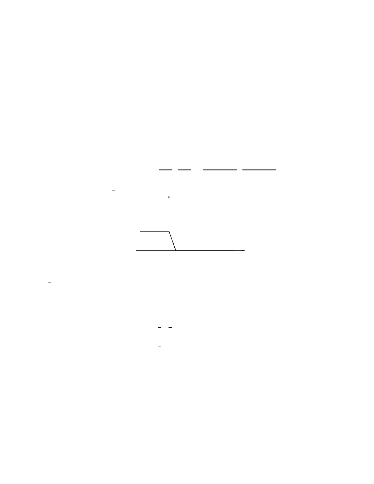
We can define φδ (s) as in the following plot, and control the error P(y · f (x) ≤ 0) in terms of Eφδ (y ·f (x)):
P(y · f (x) ≤ 0) = Ex,y I(y ·f (x) ≤ 0)
≤ Ex,y φδ (y · f (x))
= Eφδ (y ·f (x))
Enφδ (y ��
· f (x)) �
E(y · f (x)) − ��
Enφδ (y · f (x))) �
observed error generalization capability
n where Enφδ (y · = (^) n
1 f (x)) (^) i=1 f (x)).
� �^
φδ (y ·
s
ϕ (s)
δ
Let us define φδ (yF)
� = {φδ (y· f (x)) : f ∈ F}. The function φδ satisfies Lipschetz condition |φδ (a) − φδ (b)| ≤
1 δ |a^ −^ b|.^ Thus^ given^ any^ {zi^ = (xi, yi)}i=1,···^ ,n,
n
dz (φδ (y f (x)), φδ (y g(x))) =
1 �^
(φδ (yif (xi)) − φδ (yi · g(xi)))
2 · · ,definition of dz n i= � � 1 / 2 n 1 1 � ≤ δ n
(yif (xi) − yi · g(xi))
2 ,Lipschetz condition
i=
1 = dx(f (x), g(x)) ,definition of dx, δ
and the packing numbers for φδ (yF) and F satisfies inequality D(φδ (yF), �, dz ) ≤ D(F, � ·δ, dx).
Recall that for a VC-subgraph class H, the packing number satisfies D(H, �, dx) ≤ C(
1 )
V , where C is
a constant, and V is a constant. For its corresponding VC-hull class, there exists K(C, V ), such that
log D(F = conv(H), �, dx) ≤ K(
1 )
2 V Thus log D(φδ (yF), �, dz ) ≤ log D(F, � δ, dx) ≤ K(
1 )
2 V V +2 (^). V + (^). � ·^ � δ·
On the other hand, for a VC-subgraph class H, log D(H, �, dx) ≤ KV log
2 , where V is the VC dimension of
We proved that log D(Fd = convdH, �, dx V d log
2
. Thus log D(φδ (yFd), �, dx V d log
2 H. ) ≤ K · · (^) � ) ≤ K · · �δ.
48
Lecture 19 Generalization error bound for VC-hull classes. 18.
Remark 19.1. For a VC-subgraph class H, let V is the VC dimension of H. The packing number satisfies
� �V D(H, �, dx) ≤ k �
log k �
. D Haussler (1995) also proved the following two inequalities related to the packing
number: D(H, �, � · � 1 ) ≤
k �
�V
, and D(H, �, dx) ≤ K
1 �
�V
Since conv(H) satisfies the uniform entroy condition (Lecture 16) and f ∈ [− 1 , 1]
X , with a probability
of at least 1 − e−u^ ,
� � 2 V^ �
K
� √Eφδ 1 V^ +2^ Eφδ · u Eφδ (y · f (x)) − Enφδ (y · f (x)) ≤ √ n 0 � δ
d� + K · n
1 V 1 Eφδ · u (19.1) = Kn
− (^2) δ
− (^) V + (Eφδ ) V^ +2^ + K n
for all f ∈ F = convH. The term Eφδ to estimate appears in both sides of the above inequality. We give a
bound Eφδ ≤ x
∗ (Enφδ , n, δ) as the following. Since
Eφδ ≤ Enφδ
1 V 1 1 V^ +2^ V Eφδ ≤ Kn
− (^2) δ
− (^) V + (Eφδ ) V^ +2^ Eφδ ≤ Kn
− (^2) V + δ
− (^) V +
�
u u Eφδ ≤ K
Eφδ · Eφδ ≤ K , n
n
It follows that with a probability of at least 1 − e
−u ,
1 V^ +2^ V u (19.2) Eφδ ≤ K · (Enφδ + n
− (^2) V + δ
− (^) V +
n
for some constant K. We proceed to bound Eφδ for δ ∈ {δk = exp(−k) : k ∈ N}. Let exp(−uk) =
1 e−u k+
, it follows that uk = u + 2 log(k + 1) = u + 2 log(log δ
1 k
· + 1). Thus with a probability of at least � � 2
k∈N exp(−uk) = 1^ −^
1 e−u^ = 1 −
π^2 1 − (^) k∈N e−u^ < 1 − 2 e−u^ , k+1 6
1 V^ +2^ V^ V +1 uk Eφδ^2 k (y^ ·^ f^ (x))^ ≤^ K^ ·^ (Enφδk (y^ ·^ f^ (x))^ +^ n
− (^) V + δk
−
n
1 V +2 (^) VV + (19.3) = K (Enφδk (y f (x)) + n
− (^2) V + δk
−
u + 2 · log(log (^) δ
1 k
n
for all f ∈ F and all δk ∈ {δk : k ∈ N}. Since P(y · f (x) ≤ 0) = Ex,y I(y · f (x) < 0) ≤ Ex,y φδ (y ·f (x)), and
Enφδ (y f (x)) = (^) n
1 n i=1 φδ^ (yi^ ·^ f^ (xi))^ ≤^ n
1 n · i=1 I(yi · f (xi) ≤ δ) = Pn(yi · f (xi) ≤ δ), with probability at
least 1 − 2 e
−u · ,
V +2 (^) V u 2 log(log 1 + 1) P(y · f (x)) ≤ 0) ≤ K · inf δ
Pn(y · f (x) ≤ δ) + n
− (^) 2(V +1) δ
− (^) V +
n
n
δ .