Download Electrostatics: Potential & Surface Charges with Line Charges & Conducting Sphere and more Assignments Physics in PDF only on Docsity!
Physics 505 Fall 2005
Homework Assignment #2 — Solutions
Textbook problems: Ch. 2: 2.3, 2.4, 2.7, 2.
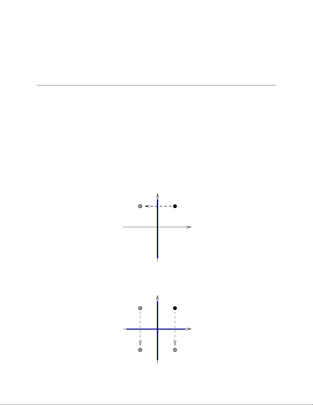
2.3 A straight-line charge with constant linear charge density λ is located perpendicular to the x-y plane in the first quadrant at (x 0 , y 0 ). The intersecting planes x = 0, y ≥ 0 and y = 0, x ≥ 0 are conducting boundary surfaces held at zero potential. Consider the potential, fields, and surface charges in the first quadrant. a) The well-known potential for an isolated line charge at (x 0 , y 0 ) is Φ(x, y) = (λ/ 4 π� 0 ) ln(R^2 /r^2 ), where r^2 = (x − x 0 )^2 + (y − y 0 )^2 and R is a constant. De- termine the expression for the potential of the line charge in the presence of the intersecting planes. Verify explicitly that the potential and the tangential electric field vanish on the boundary surfaces. The image charges for this solution may be built up one plane at a time. If there were only a plane at x = 0, then the line charge λ at (x 0 , y 0 ) will generate an image charge −λ at (−x 0 , y 0 ).
− q q
Adding a plane at y = 0 will then result in additional image charges for the above two charges: an image of the original charge giving −λ at (x 0 , −y 0 ) and an image of the initial image giving λ at (−x 0 , −y 0 ). The final picture is that of four charges, one in each quadrant (one original and three images).
− q
q − q
q
Adding up the contributions of these four charges yields
Φ(x, y) =
λ 4 π� 0
ln
R^2
(x − x 0 )^2 + (y − y 0 )^2
R^2
(x + x 0 )^2 + (y + y 0 )^2
− ln
R^2
(x − x 0 )^2 + (y + y 0 )^2
− ln
R^2
(x + x 0 )^2 + (y − y 0 )^2
λ 4 π� 0
ln
[(x − x 0 )^2 + (y + y 0 )^2 ][(x + x 0 )^2 + (y − y 0 )^2 ] [(x − x 0 )^2 + (y − y 0 )^2 ][(x + x 0 )^2 + (y + y 0 )^2 ]
Note that the arbitrary constant R drops out of this expression. We may check the validity of this solution by evaluating the potential on the boundary surface x = 0 (y = 0 is obviously similar)
Φ(0, y) =
λ 4 π� 0
ln
[x^20 + (y + y 0 )^2 ][x^20 + (y − y 0 )^2 ] [x^20 + (y − y 0 )^2 ][x^20 + (y + y 0 )^2 ]
λ 4 π� 0
ln 1 = 0
For the tangential electric field, we may compute Ey and examine its behavior on the surface x = 0. Before setting x = 0, however, we find
Ey (x, y) = −∂y Φ(x, y) =
λ 2 π� 0
y − y 0 (x − x 0 )^2 + (y − y 0 )^2
y + y 0 (x + x 0 )^2 + (y + y 0 )^2
−
y + y 0 (x − x 0 )^2 + (y + y 0 )^2
y − y 0 (x + x 0 )^2 + (y − y 0 )^2
Finally, setting x = 0 yields
Ey (0, y) =
λ 2 π� 0
y − y 0 x^20 + (y − y 0 )^2
y + y 0 x^20 + (y + y 0 )^2
−
y + y 0 x^20 + (y + y 0 )^2
y − y 0 x^20 + (y − y 0 )^2
The result is similar for the y = 0 surface.
b) Determine the surface charge density σ on the plane y = 0, x ≥ 0. Plot σ/λ versus x for (x 0 = 2, y 0 = 1), (x 0 = 1, y 0 = 1), and (x 0 = 1, y 0 = 2). The surface charge density on the y = 0 plane is obtained from the normal component of the electric field, σ = � 0 Ey (x, 0). Setting y = 0 in (2) gives
σ =
λ 2 π
−y 0 (x − x 0 )^2 + y^20
y 0 (x + x 0 )^2 + y^20
y 0 (x − x 0 )^2 + y 02
−y 0 (x + x 0 )^2 + y 02
λy 0 π
(x + x 0 )^2 + y^20
(x − x 0 )^2 + y^20
4 λx 0 y 0 π
x [(x − x 0 )^2 + y^20 ][(x + x 0 )^2 + y 02 ] (3)
Interpret. Here we simply need to Taylor expand the expression in (1). We start by expand- ing the squares and dividing out by ρ^2 to obtain
λ 4 π� 0
ln
[1 − 2 xx ρ 2 0 + 2 yy ρ 2 0 + ρ
(^20) ρ^2 ][1 +^
2 xx 0 ρ^2 −^
2 yy 0 ρ^2 +^
ρ^20 ρ^2 ] [1 − 2 xx ρ 2 0 − 2 yy ρ 2 0 + ρ
(^20) ρ^2 ][1 +^
2 xx 0 ρ^2 +^
2 yy 0 ρ^2 +^
ρ^20 ρ^2 ]
Assuming x and y are both of O(ρ) and x 0 and y 0 are of O(ρ 0 ), we see that xx 0 /ρ^2 and yy 0 /ρ^2 are of O(ρ 0 /rho). This lets us keep track of the expansion in orders of ρ 0 /rho. Expanding up to second order gives
λ 4 π� 0
ln
1 + 2 ρ
(^20) ρ^2 −^
4 x^2 x^20 ρ^4 −^
4 y^2 y^20 ρ^4 +^
8 xyx 0 y 0 ρ^4 +^ O(^
ρ^40 ρ^4 ) 1 + 2 ρ
(^20) ρ^2 −^
4 x^2 x^20 ρ^4 −^
4 y^2 y^20 ρ^4 −^
8 xyx 0 y 0 ρ^4 +^ O(^
ρ^40 ρ^4 )
=
λ 4 π� 0
ln
16 xyx 0 y 0 ρ^4
4 λxyx 0 y 0 π� 0 ρ^4
This is basically a two-dimensional quadrupole potential, which is not too sur- prising as the space is divided into four quadrants (with alternating positive and negative (image) charges). Going to polar coordinates (x, y) = ρ(cos ϕ, sin ϕ), we have Φ ≈
2 λx 0 y 0 π� 0
sin 2ϕ ρ^2 Note that 4λx 0 y 0 is essentially the quadrupole moment (charge times area) and that the sin 2ϕ angular behavior is obviously quadrupolar (angular momentum l = 2).
2.4 A point charge is placed a distance d > R from the center of an equally charged, isolated, conducting sphere of radius R. a) Inside of what distance from the surface of the sphere is the point charge attracted rather than repelled by the charged sphere? The potential for a point charge in the presence of a charged conducting sphere is given by Φ = kq
|~x − ~y |
R/d |~x − (R/d)^2 ~y |
λ + R/d |~x |
where we have changed the notation to conform to this problem. Note that we take the charge of the sphere to be Q = λq. Here λ = 1, but in part c) below we will take λ = 2 and λ = 1/2 as well. The force is simply computed from Coulomb’s law between the charge q and the two images F = kq^2
R/d d^2 (1 − (R/d)^2 )^2
1 + R/d d^2
(in the radial direction). If we let ξ = R/d (always less than 1) we may rewrite the above as F =
kq^2 R^2
ξ^2 (λ − 2 λξ^2 − 2 ξ^3 + λξ^4 + ξ^5 ) (1 − ξ^2 )^2
Far away from the sphere (ξ → 0) the force limits to
F ≈
kq^2 R^2
λξ^2 =
kqQ d^2 which is the expected result. This is repulsive for like sign charges. On the other hand, as ξ → 1 (near the surface of the sphere) the force always becomes attractive. The neutral position between attraction and repulsion is reached when the force becomes zero, or
λ − 2 λξ^2 − 2 ξ^3 + λξ^4 + ξ^5 = 0 (5)
In general, this can only be solved numerically. However note that for λ = 1 (equal charges), this factors as
(1 − ξ − ξ^2 )(1 + ξ − ξ^3 ) = 0
Only the first factor changes sign. Solving the quadratic equation gives ξ = (
5 − 1)/2 or d R
b) What is the limiting value of the force of attraction when the point charge is located a distance a (= d − R) from the surface of the sphere, if a � R? We may approach this problem by taking ξ = 1 − a/R and letting a � R so that ξ → 1. Taking this limit in (4) will yield the correct result. However it is easier to see that for a � R the radius of curvature of the sphere can be ignored, and this problem is similar to a point charge near a conducting plane. The image charge is then −q located a distance a behind the surface, and the Coulomb force is simply
F = −
kq^2 (2a)^2
c) What are the results for parts a) and b) if the charge on the sphere is twice (half) as large as the point charge, but still the same sign? The result of part b) is independent of the charge on the sphere, and remains unchanged. On the other hand, the neutral position is given by solving (5) numerically. For λ = 2 (sphere is twice the charge) and λ = 1/2 (half the charge) we find λ = 2 :
d R
λ = 12 :
d R
Note that the boundary conditions are azimuthally symmetric. Hence the φ dependence can be eliminated by taking φ′^ → φ′^ + φ. This results in
Φ(ρ, z) =
V z 2 π
∫ (^2) π
0
dφ′
∫ (^) a
0
ρ′dρ′^
[ρ^2 + ρ′^2 − 2 ρρ′^ cos φ′^ + z^2 ]^3 /^2
c) Show that, along the axis of the circle (ρ = 0), the potential is given by
Φ = V
z √ a^2 + z^2
The integral expression (7) simplifies for ρ = 0
Φ(0, z) =
V z 2 π
∫ (^2) π
0
dφ′
∫ (^) a
0
ρ′dρ′^
(ρ′^2 + z^2 )^3 /^2
= V z
∫ (^) a 2
0
1 2 dρ
′ (^2) (ρ′ (^2) + z (^2) )− 3 / (^2) = −V z(ρ′ (^2) + z (^2) )− 1 / 2
a^2 0
= V
z (z^2 + a^2 )^1 /^2
d) Show that at large distances (ρ^2 + z^2 � a^2 ) the potential can be expanded in a power series in (ρ^2 + z^2 )−^1 , and that the leading terms are
Φ =
V a^2 2
z (ρ^2 + z^2 )^3 /^2
[
3 a^2 4(ρ^2 + z^2 )
5(3ρ^2 a^2 + a^4 ) 8(ρ^2 + z^2 )^2
]
Verify that the results of parts c) and d) are consistent with each other in their common range of validity. Returning to expression (7), we may pull out the factor r^2 = ρ^2 + z^2 and expand the denominator
V z 2 πr^3
∫ (^2) π
0
dφ′
∫ (^) a
0
ρ′dρ′
[
2 ρρ′ r^2
cos φ′^ +
ρ′^2 r^2
]− 3 / 2
V z 2 πr^3
∫ (^2) π
0
dφ′
∫ (^) a
0
ρ′dρ′
[
1 − 32 r−^2 (ρ′^2 − 2 ρρ′^ cos φ′)
- 158 r−^4 (ρ′^2 − 2 ρρ′^ cos φ′)^2 + · · ·
]
The φ′^ integral is now trivial (since it is over a complete period) and pulls out terms with even powers of cos φ′. The resulting integral is
Φ(ρ, z) =
V z r^3
∫ (^) a^2
0
1 2 dρ
′ 2 [1 − 3
2 r
− (^2) ρ′ (^2) + 15 8 r
− (^4) (ρ′ (^4) + 2ρ (^2) ρ′ (^2) ) + · · ·]
V z 2 r^3
[a^2 − 34 r^2 a^4 + 158 r−^4 ( 13 a^6 + ρ^2 a^4 ) + · · ·]
V a^2 2
z (ρ^2 + z^2 )^3 /^2
[
3 4 a
2 ρ^2 + z^2
5 8 a
(^2) (3ρ (^2) + a (^2) ) (ρ^2 + z^2 )^2
]
Setting ρ = 0 in this series gives
Φ(0, z) =
V a^2 2 z^2
[
a^2 z^2
a^4 z^4
]
On the other hand, the exact potential on axis, (8), may be expanded
Φ(0, z) = V
[
a^2 z^2
)− 1 / 2 ]
= V
[
a^2 z^2
a^4 z^4
a^6 z^6
)]
V a^2 2 z^2
[
a^2 z^2
a^4 z^4
]
This agrees with the series (9).
2.10 A large parallel plate capacitor is made up of two plane conducting sheets with sepa- ration D, one of which has a small hemispherical boss of radius a on its inner surface (D � a). The conductor with the boss is kept at zero potential, and the other con- ductor is at a potential such that far from the boss the electric field between the plates is E 0. a) Calculate the surface-charge densities at an arbitrary point on the plane and on the boss, and sketch their behavior as a function of distance (or angle). The way to approach this problem is to realize that the second conductor (the one without the boss) is kept far away from the region of interest (which is near the boss). As a result its only real purpose is to complete the capacitor and create a nearly uniform electric field E 0. As a result, this problem reduces to that of a conductor with a hemispherical boss in a uniform electric field. This, in turn, can be seen to be equivalent to half of the space of the conducting sphere in a uniform electric field setup.
E 0
D
z
a
Taking the conductor to be located at z = 0, the boss to be located at the origin, and the space between the plates to be z > 0, we end up with the (sphere in a uniform field) potential
Φ = −E 0 z
a^3 r^3
0 < z < D
c) If, instead of the other conducting sheet at a different potential, a point charge q is placed directly above the hemispherical boss at a distance d from its center, show that the charge induced on the boss is
q′^ = −q
[
d^2 − a^2 d
d^2 + a^2
]
Taking away the second conductor (i.e. removing the electric field) turns this into an image charge problem for a point charge near a conducting sphere. For the sphere by itself, a charge q at position d generates an image −q(a/d) at location a^2 /d. Starting from this, we introduce the conducting plane at z = 0. This gives additional image charges based on the reflection z → −z. The images of the original charge and first image are thus −q and −d and q(a/d) and −a^2 /d. In other words
Φ(~x ) = kq
|~x − dzˆ|
a/d |~x − (a^2 /d)ˆz|
|~x + dˆz|
a/d |~x + (a^2 /d)ˆz|
The surface charge on the boss is given by σ = −� 0 xˆ · ∇~Φ|x=a, which has for the most part been calculated several times before in the spherical conductor examples. The result for (10) is
σ = −� 0 kq
d^2 − a^2 a(d^2 + a^2 − 2 ad cos θ)^3 /^2
d^2 − a^2 a(d^2 + a^2 + 2ad cos θ)^3 /^2
q 4 πa
(d^2 − a^2 )
(d^2 + a^2 − 2 ad cos θ)^3 /^2
(d^2 + a^2 + 2ad cos θ)^3 /^2
The total charge on the boss is given by integration
Qboss = −
q 4 πa
(d^2 − a^2 )(2πa^2 )
0
d cos θ
(d^2 + a^2 − 2 ad cos θ)^3 /^2
−
(d^2 + a^2 + 2ad cos θ)^3 /^2
q 2 d
(d^2 − a^2 )
[
(d^2 + a^2 − 2 ad cos θ)−^1 /^2 + (d^2 + a^2 + 2ad cos θ)^1 /^2
] 1
0
= −
q 2 d
(d^2 − a^2 )
d − a
d + a
(d^2 + a^2 )^1 /^2
= −q
d^2 − a^2 d(d^2 + a^2 )^1 /^2