In-Class Activity #8: Pivot Tables and Charts Tutorial
(Due Monday, March 20, 9:00 am)
Submission Guideline:
o Submit a single WORD/PDF file for Questions 1, 2, 3 and 4.
o The file should include: (1) the answers to each question, and
o (2) the Pivot Table or Pivot Chart (unless otherwise specified) created to answer the question.
This tutorial provides an overview of creating pivot tables and pivot charts in Microsoft Excel. The screenshots are
from Office 2013. Things may look a little different if you have an earlier version (or the Mac version!) of Excel.
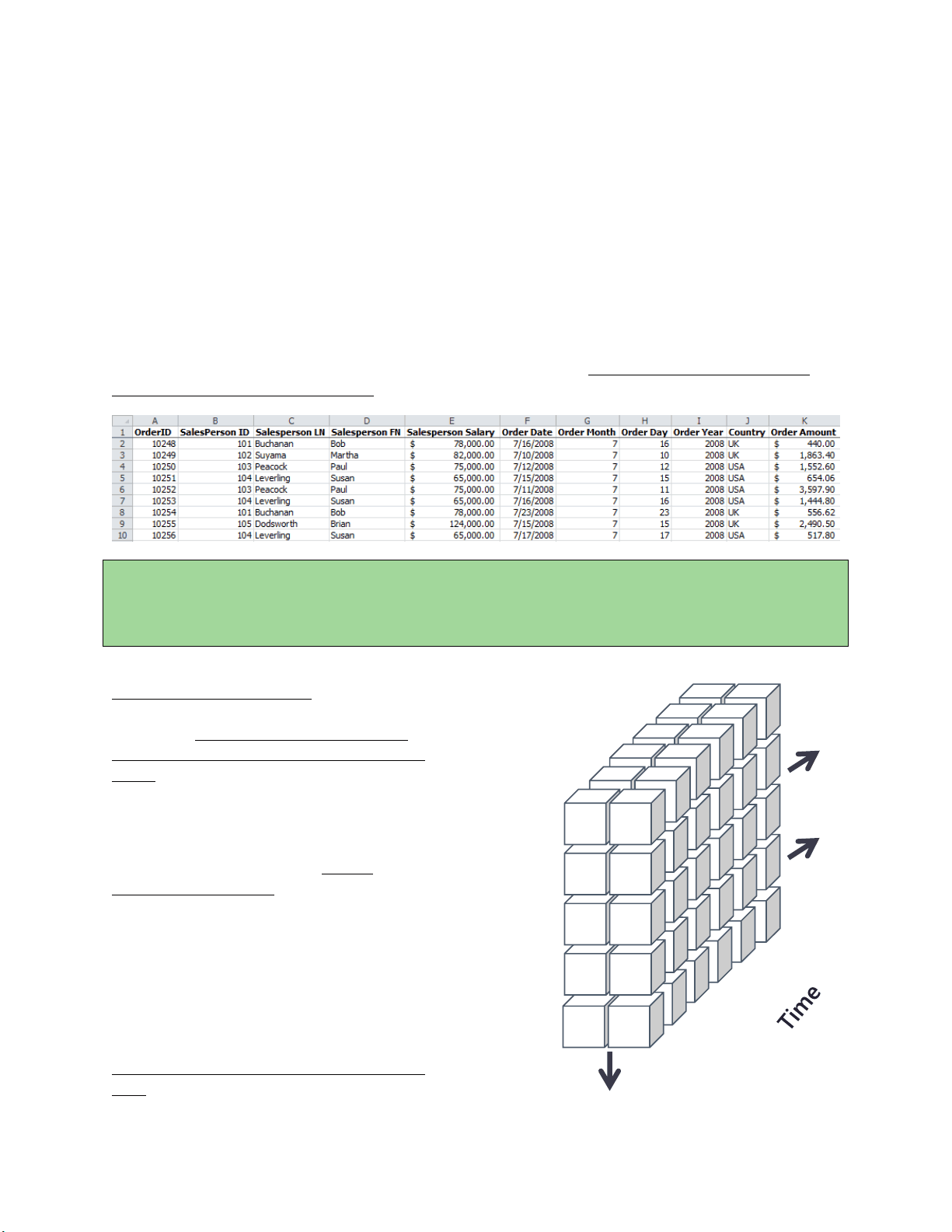
First, let’s look at the data cube with which we will be working. The data cube is contained in the file “In-Class
Exercise #8 - Salesperson Cube - for class.xlsx.” There is information about 800 sales transactions that occurred
from 2008 to 2010 at a fictitious company. Here are the first few records:
Keep in mind that this is the entire data set in a joined, cube format. It’s not a typical, large -scale data cube – that
would only contain summary data. In this tutorial, you’ll be basically doing the summarization work of the
dimensional engine by aggregating data as you need it. This works well for small data sets and gives you a lot of
flexibility, but as your data set gets very large this would need to be implemented as a summarized cube.
The underlying star schema has three dimensions –
Salesperson, Country, and Time. You can see data
associated with each of those dimensions. For
example, the Salesperson dimension consists of
Salesperson LN, Salesperson FN, and Salesperson
Salary.
So a diagram of our data cube looks would look like
the image on the right.
There are only two values for the Country
dimension (USA and UK), but there are a lot for
Salesperson and Time. In fact, there are too many to
draw so we’ve used arrows to indicate that the cube
keeps going in that direction for a while. But this
gives you a feel for the structure of our data mart,
and it also indicates to us that we will be able to
aggregate and filter our results by salesperson, time,
and country.
Notice time is expressed two different ways in our
table. The first is with day, month, and year as
separate attributes; the second as a standard date/time value (mm/dd/yyyy). It isn’t necessary to do this – a single
Order
amount
Order
amount
Order
amount
Order
amount
Order
amount
Order
amount
Order
amount
Order
amount
Order
amount
Country
Salesperson
USA
Bob
Buchanan
Martha
Suyama
Paul
Peacock
Susan
Leverling
7/10/2008
Order
amount
UK
7/11/2008
7/12/2008
7/15/2008
7/16/2008
7/17/2008
Susan
Leverling
…more
salespeople
…more time
periods