Economics 310
Handout # VI Limited Dependent Variable Models
I. Binary Choice Models
A. Linear Probability Model
B. Probit Model (See: Economics 210 handouts)
C. Logit Model
II. Multiple Choice Models
A. Ordered Probit and Logit Models
B. Multinomial Logit Model
C. Conditional Logit Model
D. Poission Model (Count data)
III. Truncated Dependent Variable Models
A. Tobit Model (See: Tobit model handout)
B. Sample Selection Model
IIA. The Ordered Probit and Logit Models
Frequently a dependent variable takes on several unambiguously ordered values. For example,
suppose we consider bond ratings AAA, AA, A, etc. AAA is unambiguously a better rating than
AA and AA is unambiguously a better rating than A and so forth. Other examples would be the
ratings of various goods from consumer surveys, the ranking of politicians from opinion polls,
results from opinion poll on issues (strongly agree, agree, no opinion, disagree, strongly
disagree), levels of education (elementary school, high school, college, graduate study), levels of
employment (unemployed, part time, full time) and levels of risk for insurance. Note that in
each of these cases the ordering is unambiguous.
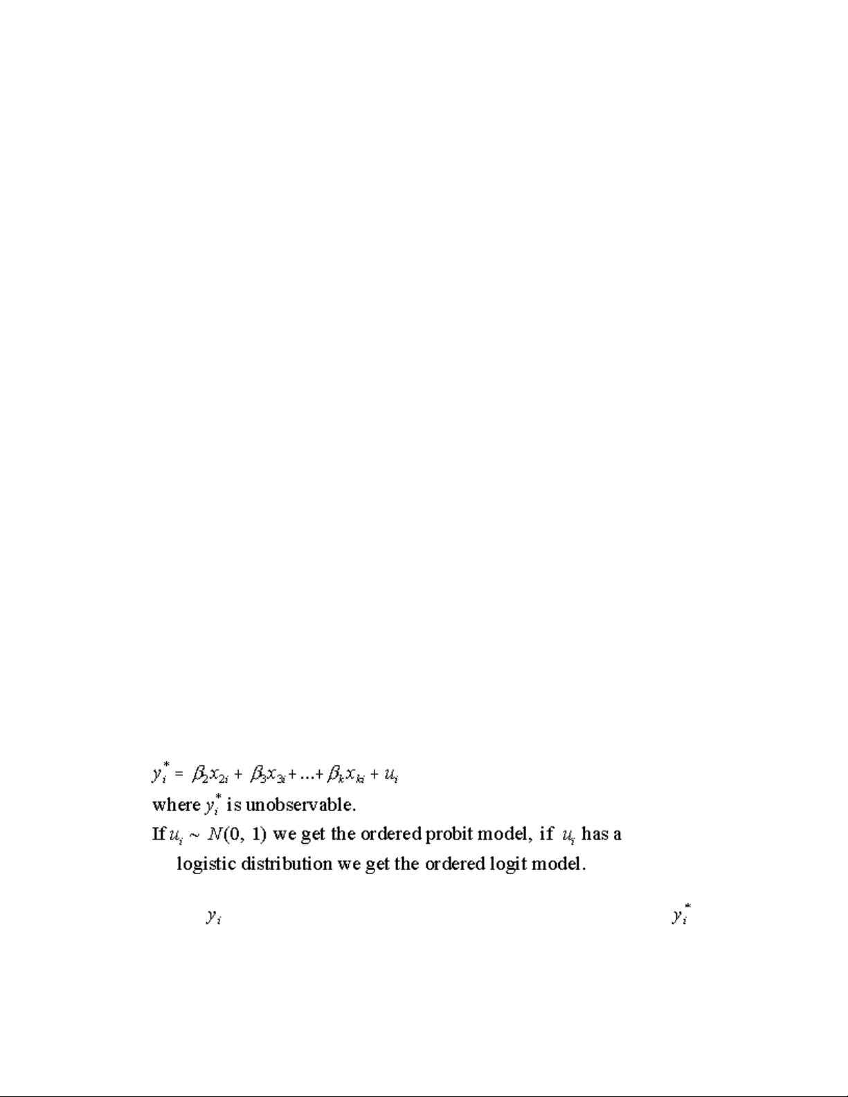
The Model
We assume that takes on one of the values 0, 1, 2, ..... J depending on the value of .