Download Price Discrimination - Intermediate Microeconomics - Lecture Slides and more Slides Microeconomics in PDF only on Docsity!
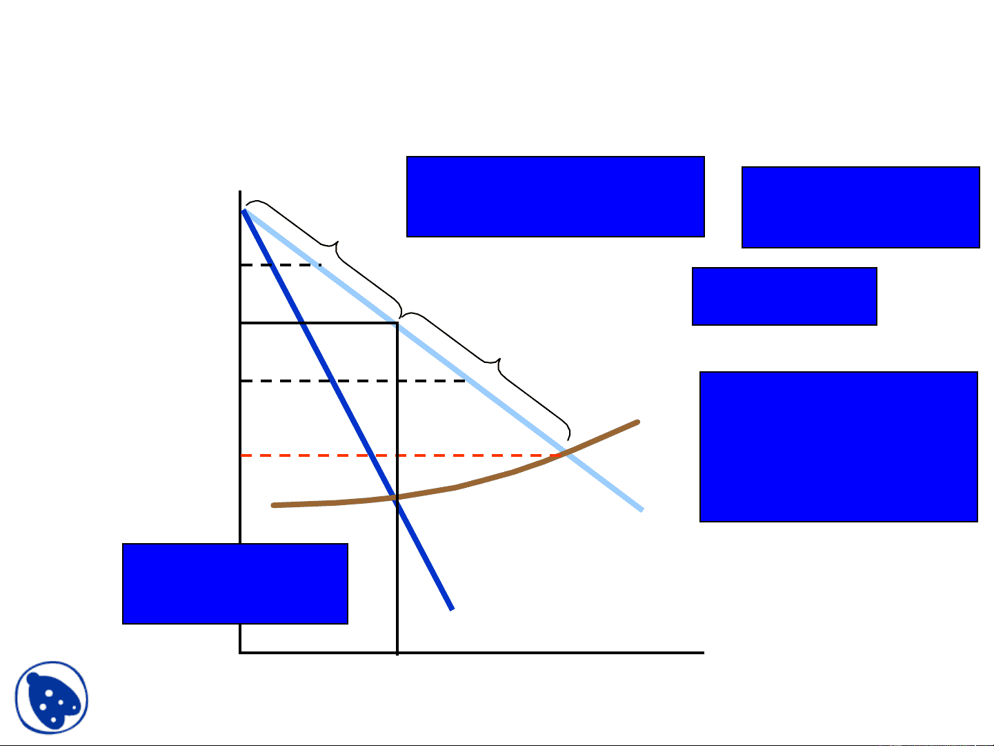
Price Discrimination: Capturing CS
Quantity
$/Q
D
MR
Pmax
MC
If price is raised above P*, the firm will lose sales and reduce profit.
PC
PC is the perfectly competitive price.
A
_P_*
Q*
P 1
Between 0 and Q, consumers will pay more than P--consumer surplus (A).
B
P 2
Beyond Q*, price will have to fall to get at consumer surplus (B).
• PQ: MC = MR
- A: CS with _P_*
- B: P>MC ; consumer would buy at a lower price
- P 1 : less sales and π
- P 2 : increase sales; ↓π
First-Degree (Perfect) Price Discrimination
P*
Q*
Without price discrimination, output is Q* and price is P*. Variable profit is the area between the MC & MR (yellow).
Quantity
$/Q P
max
Each consumer pays their reservation (maximum) price: Profits Increase
Consumer surplus is the area above P* and between 0 and Q* output.
D = AR
MR
MC
Output expands to Q** and price falls to PC where MC = MR = AR = D. Profits increase by the area above MC between old MR and D to output Q** (purple)
Q**
PC
Second-Degree Price Discrimination
Quantity
$/Q
D
MR
MC
AC
P 0
Q 0
Without discrimination: P = P 0 and Q = Q 0. With second-degree discrimination there are three prices P 1 , P 2 , and P 3. (e.g. electric utilities)
P 1
Q 1
1st Block
P 2
Q 2
P 3
Q 3
2nd Block 3rd Block
Second-degree price discrimination is pricing according to quantity consumed--or in blocks.
docsity.com
Third Degree Price Discrimination
Divides the market into two-groups.
Each group has its own demand function.
Most common type of price discrimination.
- Examples: airlines, liquor, vegetables, discounts to students and senior citizens.
- Feasible when the seller can separate his/her
market into groups who have different price elasticities
of demand (e.g. business air travelers versus vacation air
travelers)
Third-Degree Price Discrimination
Quantity
D 2 = AR 2
MR 2
$/Q
MR^ D^1 = AR^1
1
Consumers are divided into two groups, with separate demand curves for each group.
MRT
MRT = MR 1 + MR 2
Third-Degree Price Discrimination
Quantity
D 2 = AR 2
MR 2
$/Q
MR^ D^1 = AR^1
1
MRT
MC
Q 2
P 2
QT
• QT: MC = MRT
- Group 1: P 1 Q 1 ; more inelastic
- Group 2: P 2 Q 2 ; more elastic
- MR 1 = MR 2 = MC
- MC depends on QT
Q 1
P 1
Airline Fares
• Differences in elasticities imply that some customers will
pay a higher fare than others.
• Business travelers have few choices and their demand is
less elastic.
• Casual travelers have choices and are more price sensitive.
• The airlines separate the market by setting various
restrictions on the tickets.
- Less expensive: notice, stay over the weekend, no refund
- Most expensive: no restrictions
Intertemporal Price Discrimination
- Separating the Market With Time
- Initial release of a product, the demand is inelastic
- Once this market has yielded a maximum profit, firms
lower the price to appeal to a general market with a more
elastic demand
- Paper back books, Dollar Movies, Discount computers
Peak-Load Pricing
- Demand for some products may peak at particular times.
E.g. Rush hour traffic, Electricity - late summer afternoons,
Ski resorts on weekends
- Capacity restraints will also increase MC.
- Increased MR and MC would indicate a higher price.
- MR is not equal for each market because one market does
not impact the other market.
Peak-Load Pricing
Peak-Load Pricing
MR 1
D 1 = AR 1
MC
P 1
Q 1
Peak-load
price = P 1.
Quantity
$/Q
MR 2
D 2 = AR 2
Off- load
price = P 2.
Q 2
P 2
Two-Part Tariff with a Single Consumer
Usage price P* is set where
MC = D. Entry price T*
is equal to the entire
consumer surplus.
T*
Quantity
$/Q
MC
P*
D
Two-Part Tariff with Two Consumers
D 2 = consumer 2
D 1 = consumer 1
Quantity
$/Q
MC
A
B
C
morethan twiceABC
2 ( ) ( 1 2 )
T P MC x Q Q
Q 2 Q 1
The price, _P,_* will be greater than MC. Set _T_*
T* at the surplus value of D2.
P*