Download Implementing Systolic Arrays using Verilog: A Parallel Approach to Matrix Vector Products and more Study Guides, Projects, Research Computer Architecture and Organization in PDF only on Docsity!
Project 3: Implementing Systolic Arrays using Verilog
University of Central Florida
School of Electrical Engineering and Computer Science
CDA 4150 Computer Architecture
Fall 2005 (Due 12/1/05)
An alternative to solve the matrix vector product in parallel are systolic arrays. The name sys- tolic array was proposed by Kung and Leiserson to a network of processing elements that act synchronously to solve specific problems. These networks of processing elements exploit pipelining, parallel processing, and use simple and regular communication paths. At each computation step the processing elements of the systolic array get data, either from another processing element(s) or from outside the network, execute some computation, and pump data out either outside the network or to another processing element(s). The name systolic was proposed by analogy with the way the heart pumps blood through the circulatory system and the manner systolic array pumps data in and out the processing elements.
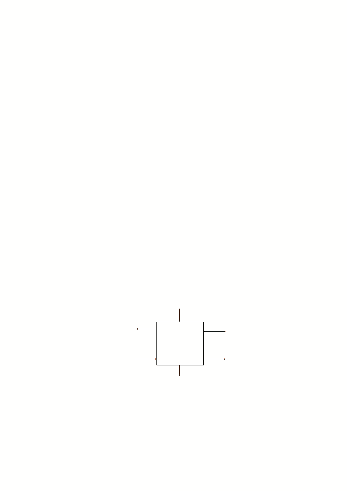
The systolic array proposed by Kung and Leiserson, in the late seventies, to compute the band matrix vector product is the one we will used through this work and we will refer to it as Kung’s Systolic Array (KSA). The basic processing element of KSA is the Inner-Product-Step-Processor (IPSP), which is depicted in Figure 1. An IPSP has three inputs ports and three output ports and is defined as follows:
IP SP (a, x, y) → (a, x, y + a × x)
y + a * x
x x
y
a
a Figure 1: data flow in a systolic processing element.
We will explain how a KSA with three processing elements computes the band matrix vector product
y 1 y 2 y 3 y 4
=
a 11 a 12 0 0 a 21 a 22 a 11 0 0 a 32 a 33 a 34 0 0 a 43 a 144
x 1 x 2 x 3 x 4
using the following recurrences:
y i^1 = 0, y ik +1= yik + aik × xk, yi = y in+
As in KSA the matrix must enter the systolic array by diagonals the number of processing elements required is equal to the number of diagonals w = 3 of matrix A. In Figure 2, we show how the components of the vector x enter the systolic array from left to right, the components of the vector y, initially zero, enter the systolic array from right to left, and the coefficients of the matrix A will enter the systolic array, by diagonals, from top to bottom. At each step of the computation three values enter in each IPSP, a computation is executed, each yi accumulates its partial result, and three values are pumped out. This computation requires w steps to move the first component y 1 to the leftmost processing element and then, as the components of vector y enter the array every other unit of time, 2n − 1 additional steps are necessary to pump out all the elements of the resulting vector y for an overall of T (n) = w + 2n − 1. The first five steps of the of the computation are shown in Figure 3, where it can be observed that each processing element of the systolic array is working on the matrix vector product on every other unit of time.
a 44
a 34 a 43
a 33
a 23 a 32
a 22
a 12 a 21
a 11
Y 1 Y (^2) X (^1) Figure 2: Kung’s Systolic array to compute a band matrix vector product.
Surprisingly, the same linear systolic array computes two matrix vector products simultaneously in T (n) = w + 2n steps using perfect shuffling as a spatial data scheduling technique. Therefore,
Where the symbols | 0 〉 and | 1 〉, are known as ket zero and ket one according to Dirac’s notation.
To move a state vector from one state to another we must use unitary transformations which are represented by 2 × 2 matrices and we will refer to them as unitary operations or gates. As an example, we show the unitary operations Identity(I), NOT(X) and Hadamard(H): The identity gate just left the state vector as is:
I| 0 〉 =
[ 1 0 0 1
] [ 1 0
]
[ 1 0
] = | 0 〉
I| 1 〉 =
[ 1 0 0 1
] [ 0 1
]
[ 0 1
] = | 1 〉
the X gate flips | 0 〉 into | 1 〉 and vise versa:
X| 0 〉 =
[ 0 1 1 0
] [ 1 0
]
[ 0 1
] = | 1 〉
X| 1 〉 =
[ 0 1 1 0
] [ 0 1
]
[ 1 0
] = | 0 〉
and the Hadamard (H) gate turns | 0 〉 and | 1 〉 into a equally weighted superposition state. The H gate is defined as
H = √^12
[ 1 1 1 − 1
]
and when it is applied to | 0 〉 and | 1 〉 we obtain the following superposition:
H| 0 〉 = √^12
[ 1 1 1 − 1
] [ 1 0
]
[ 1 1
]
H| 0 〉 = √^12
[ 1 1 1 − 1
] [ 0 1
]
[ 1 − 1
]
You have to implement, in Verilog, the following operations in parallel using a systolic array with three processing elements and applying the technique used in the homework:
H| 0 〉 = √^12
[ 1 1 1 − 1
] [ 1 0
]
[ 1 1
]
I| 0 〉 =
[ 1 0 0 1
] [ 1 0
]
[ 1 0
]
The input to systolic arrays is a 1-Dimensional vector denoted the carrier vector. As the I operation just left the second vector as is, we can use the value ”D”. For instance.
D
D
D
D
Where ”D” stands for a don’t care value. The 2 vectors once loaded in the carrier vector can have four possibilities. In Figure 5 we use ”D” in the second input vector:
|^11 〉^ =>
1 D 0 D
1 D 1 D 1 0
1 0
Step 1 D = don’tcare
0 1 1 0
1 1 0 0
H adam ard G ate
1 1
1 0
αβ
00 10
αβ
1 0 - 1 0 1 1 1 1
Figure 5: First step of the systolic teleportation design.
The output of the first systolic array (input for the next systolic array) has to be multiplied for two matrices in parallel according to the following rules (see Figure 6):
- If the value of the first component of the carrier vector is 0 use I||X
2.- If the value of the first component of the carrier vector is 1 use I||I
You must deliver in a CD: