spacecraft design engineering, Study notes of Space Flight Mechanics

Download spacecraft design engineering and more Study notes Space Flight Mechanics in PDF only on Docsity!

Spacecraft Mission Design

Second Edition

Spacecraft Mission Design

Second Edition

Charles D. Brown Wren Software, Inc. Castle Rock, Colorado

&AIAA

EDUCATION SERIES

J. S. Przemieniecki

Series Editor-in-Chief

Air Force Institute of Technology

Wright-Patterson Air Force Base, Ohio

Published by American Institute of Aeronautics and Astronautics, Inc. 1801 Alexander Bell Drive, Reston, VA

American Institute of Aeronautics and Astronautics, Inc., Reston, Virginia

1 2 3 4 5

Library of Congress Cataloging-in-Publication Data

Brown, Charles D., 1930- Spacecraft mission design / Charles D. Brown. — 2nd ed. p. cm. Includes bibliographical references and index. ISBN 1-56347-262-7 (alk. paper)

1. Space flight-Planning. 2. Astrodynamics. 3. ORB WIN. I. Title. TL790.B735 1998 629.4'l-dc21 98-

Copyright © 1998 by the American Institute of Aeronautics and Astronautics, Inc. All rights reserved. Printed in the United States of America. No part of this publication may be reproduced, distributed, or transmitted, in any form or by any means, or stored in a database or retrieval system, without the prior written permission of the publisher.

Data and information appearing in this book are for informational purposes only. AIAA is not responsi- ble for any injury or damage resulting from use or reliance, nor does AIAA warrant that use or reliance will be free from privately owned rights.

This page intentionally left blank

About the Author

Charles Brown has had a distinguished career as the manager of planetary space- craft projects and as a college-level lecturer in spacecraft design. During his 30 years with Martin Marietta, he led the design team that produced propulsion sys- tems for Mariner 9 and Viking Orbiter. Among other projects, he directed the team that produced the successful Venus-imaging spacecraft, Magellan. Magellan was launched on Space Shuttle Atlantis in 1989 and completed the first global map of the surface of Venus. Magellan was the first planetary spacecraft to fly on the Shuttle and the first planetary launch by the United States in 10 years. Mr. Brown has instructed a popular spacecraft design course at Colorado Uni- versity since 1981. This book was originally written for use in that course. Mr. Brown also is the author of Spacecraft Propulsion, published by AIAA, and he writes software for Wren Software, Inc., a small software company he founded in 1984. He was corecipient of the Dr. Robert H. Goddard Memorial Trophy in 1992 for Magellan leadership. He has also received the Astronauts' Silver Snoopy Award in 1989; the NASA Public Service Medal in 1992 for Magellan and in 1976 for Viking Orbiter; and the Outstanding Engineering Achievement Award, 1989 (a team award), from the National Society of Professional Engineers for Magellan.

Table of

Contents

• Chapter 1. Introduction Preface x i - 1.1 Arrangement of the Book - 1.2 ORB WIN: AIAA Mission Design Software - 1.3 Study of Two-Body Motion
• Chapter 2. Two-Body Motion
  • 2.1 Circular O r b i t s
  • 2.2 General Solution
  • 2.3 Elliptical Orbits
    • 2.4 Parabolic Orbits
  • 2.5 Hyperbolic Orbits
  • 2.6 Time Systems
  • 2.7 Coordinate Systems
  • 2.8 Classical Orbital Elements - Problems
• Chapter 3. Orbital Maneuvers
  • 3.1 In-Plane Orbit Changes
  • 3.2 Hohmann Transfer
  • 3.3 Bielliptical Transfer
  • 3.4 Plane Changes
  • 3.5 Combined Maneuvers
  • 3.6 Propulsion for Maneuvers - Problems
• Chapter 4. Observing the Central Body
  • 4.1 Effect of the Launch Site
  • 4.2 Orbit Perturbations
  • 4.3 Ground Track
  • 4.4 Spacecraft Horizon
  • 4.5 Constellations - Problems
    • Chapter 5. Special Earth Orbits - 5.1 Geosynchronous Orbit - 5.2 Sun-Synchronous O r b i t - 5.3 Molniya Orbit - 5.4 Low Earth O r b i t - Problems
    • Chapter 6. Interplanetary Trajectories - 6.1 Patched Conic Approximation - 6.2 Highly Simplified Example - 6.3 Patched Conic Procedure - 6.4 Locating the Planets - 6.5 Design of the Transfer Ellipse - 6.6 Design of the Departure Trajectory - 6.7 Design of the Arrival Trajectory - 6.8 Gravity-Assist M a n e u v e r - 6.9 Cycler O r b i t s - 6.10 Establishing Planetary Orbit - Problems
  • Chapter 7. Lunar Trajectories - 7.1 Motion of the Earth-Moon System - 7.2 Time of Flight and Injection Velocity - 7.3 Sphere of Influence - 7.4 Lunar Patched Conic - Problems
  • Appendix A. ORBWIN: AIAA Mission Design Software - A.I Introduction to ORBWIN - A.2 Quick Tour of ORBWIN - A.3 Orbit Definition Example - A.4 Utilities - A.5 Interesting Orbits—Examples
• Appendix B. Mission Design Glossary
• Appendix C. Mission Design D a t a
• R e f e r e n c e s
• Index

1

Introduction

You need nothing more than this book and the ORB WIN software that comes with it to design a mission to anywhere in the solar system. Are you interested in how the Mars Sample Return mission will be flown? Or would you like to study a mission to Titan, one of Saturn's moons and a candidate for life? Or are you interested in the feasibility of a mission to Pluto, the last unexplored planet? Have at it.

1.1 Arrangement of the Book The first three chapters of the book describe the basic equations of two-body motion including the design of maneuvers and the special relations involved in observing the central body. Chapters 5 and 6 give examples of mission designs of several of the most important orbit types. Chapter 6 also covers the interesting complexities of interplanetary orbits and includes a detailed example. The appendices were designed to provide the working professional with ready reference material. Appendix A is the manual for ORB WIN: AIAA Mission Design Software. Appendix B is a glossary of mission design terms, which are unusually obtuse. Equations, design data, and conversion factors are in Appendix C.

1.2 ORBWIN: AIAA Mission Design Software This book includes ORBWIN: AIAA Mission Design Software. With ORBWIN you can do complete mission designs with the accuracy, speed, and downright convenience of personal computing. You no longer need to have a mainframe to do quality work in this field.

1.3 Study of Two-Body Motion Much of the history of mathematical and physical thought was inspired by cu- riosity about the motion of the planets—the very same laws that govern the motion of spacecraft. The first observations of the celestial bodies predate recorded his- tory. The inertial position of the vernal equinox vector was observed and recorded in stone constructions—Stonehenge, for example—as early as 1800 B.C. Written evidence of stellar observations was left by the Egyptians and the Babylonians from about 3500 years ago. (The Babylonians of this era divided time into 60 even units, a tradition that survives to this day. 1 ) In about 350 B.C. Aristotle explained the wandering motion of the planets by proposing that the universe was composed of 55 concentric rotating spheres cen- tered in the Earth. The outermost sphere contained the fixed stars; its rotation is a very adequate explanation of the observed motion of stars in the night sky and

2 SPACECRAFT MISSION DESIGN

the irresistible image of a celestial sphere. The rotation of the inner sphere con- taining the moon was also a simple, descriptive idea. The motion of the planets, however, was much more difficult. Not only were the observing instruments crude

and the mathematical tools nonexistent, the Earth is a singularly poor observation

post for heliocentric motion. Usually the planets move slowly eastward across a background of fixed stars; however, at times they reverse direction and move west- ward. The retrograde loop of Mars is renowned. To explain this motion, Aristotle invented the remaining 53 concentric spheres. Each planet was located in one of the spheres, and its motion was influenced by the rotation of several other spheres.^2 At about the same time a Greek named Aristarchus proposed a much simpler theory in which the sun and stars were fixed and the planets rotated about the sun, but this theory was not accepted. Aristotle's theory dominated scientific thought

for 1800 years.

In about 150 A.D. the Greek astronomer Ptolemy presented a more elaborate Earth-centered theory, which held that the planets moved around the Earth in small circles called epicycles, whose centers moved around in large circles called deferents. The tables of planetary motion computed by Ptolemy based on this theory were used for 1400 years. In 1543 Nicholas Copernicus broke with Aristotle's theory and advocated sun- centered rotation. His theory neatly explained the retrograde motion of the planets as observed from Earth; however, measured positions were so crude at the time that they fit Ptolemy's conception as well as that of Copernicus. In about 1610 the Italian scientist Galileo Galilei made two observations that reinforced the theory of Copernicus. First, he observed the motion of moons or- biting Jupiter; thus at least some bodies must not orbit Earth. Second, he observed moonlike phases of the sunlight on Venus that could not be explained by Ptolemy's theory. Galileo attracted the wrath of the Catholic Church and was forced to recant his observations. In the late 1500s Tycho Brahe made the first accurate measurements of the positions of the planets as a function of time. His achievement is all the more remarkable because the telescope had not yet been invented. Brahe himself believed

in Ptolemy's theory of the universe, but his careful observations allowed Johannes

Kepler to describe mathematically the heliocentric motion of the planets and to

lay to rest the ancient theories of Aristotle and Ptolemy.

In early 1600, Kepler presented his three laws of planetary motion, which are

the basis of our understanding of planetary (and spacecraft) motion.

First Law: The orbit of each planet is an ellipse, with the sun at one focus. Second Law: The line joining the planet to the sun sweeps out equal areas in equal times. Third Law: The square of the period of a planetary orbit is proportional to the cube of its mean radius.

In addition, Kepler contributed Kepler's equation, which relates position and time. Kepler's equation is the most famous transcendental equation ever discov- ered. Solving it for the time elapsed since periapsis when one is given orbital ele- ments is trivial; solving it for orbital elements when one is given the time elapsed since periapsis was the "Mount Everest" of mathematics for three centuries.

This page intentionally left blank

2

Two-Body Motion

All of the celestial bodies, from a fleck of dust to a supernova, are attracted to each other in accordance with Newton's law of universal gravitation: F 8 = MmG/r^2 (2.1) where

Fg = universal gravitational force between bodies M, m — mass of the two bodies G = universal gravitational constant r — distance between the center of masses of the two bodies

The motion of a spacecraft in the universe is governed by an infinite network of attractions to all celestial bodies. A rigorous analysis of this network would be impossible; fortunately, the motion of a spacecraft in the solar system is dominated by one central body at a time. This observation leads to the very useful two-body assumptions:

1. The motion of a spacecraft is governed by attraction to a single central body.
2. The mass of the spacecraft is negligible compared to that of the central body.
3. The bodies are spherically symmetric with the masses concentrated at the centers.
4. No forces act on the bodies except for gravitational forces and centrifugal forces acting along the line of centers. If the two-body assumptions hold, it can be shown that conic sections are the only possible paths for orbiting bodies and that the central body must be at a focus of the conic.^4 The two-body assumptions are very nearly true. Table 2.1 shows the most sig- nificant relative accelerations on a low Earth orbiter. The influence of Earth on the spacecraft is more significant than any other influence by more than a factor of 1000. The oblateness of the Earth also leads to errors in two-body solutions; however, these errors are small and can be accurately predicted. No explicit solution has been found for the Af-body problem except for N = 2; however, numerical solutions are available for the N-body situation. These solu- tions require a large computing capacity and are used only when the two-body solution is suspect (e.g., a Mercury orbiter) or when high accuracy is required (e.g., navigation calculations).

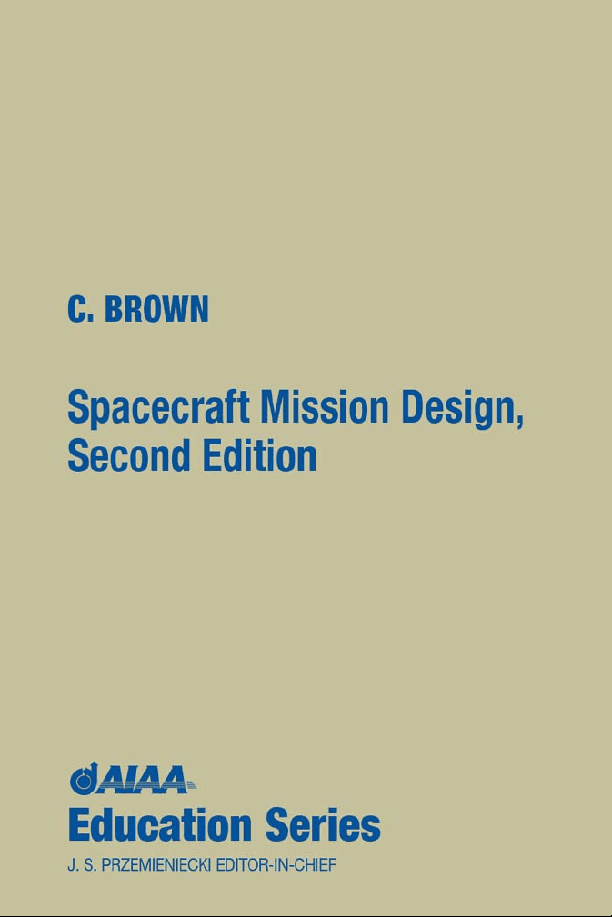
2.1 Circular Orbits

Figure 2.1 shows the forces on a spacecraft in a circular orbit under two-body conditions. The gravitational force on the spacecraft is defined by Eq. (2.1); the

TWO-BODY MOTION 7

It is convenient to assign a gravitational parameter //,, which is the product of the central body mass and the universal gravitational constant. In other words,

At = MG (2.5)

allows the simplification

V = V^/7 (2.6)

for circular orbits. The gravitational parameter is a property of the central body; a table that lists values for each of the major bodies in the solar system is given in Appendix C. (Substantial improvement in the accuracy of planetary constants is one of the by-products of planetary exploration.) The period of a circular orbit, derived with equal simplicity, is given by

P = circumference/velocity = 2;ri/r^3 /'/z (2.7)

Example 2.1 Circular Orbit Velocity and Period

What is the velocity of the Space Shuttle in a 150-n mile circular orbit? From Appendix C, for Earth,

#0 = 6378.14 km

fi = 398,600 km 3 /s 2

Spacecraft altitude h is specified more frequently than radius r in practical ap- plications. It is understood that altitude, used as an orbital element, is given with respect to the mean equatorial radius RQ. Calculate r (the conversion factor for nautical miles to kilometers is given in Table C. 10 of Appendix C):

r = R 0 + h = 6378.14 + (150)(1.852) = 6655.94 km

Calculate Shuttle velocity for a circular orbit by using Eq. (2.6):

V = ^398,600/6655.94 = 7.739 km/s

Calculate orbit period by using Eq. (2.7):

P = 27t^/r^i = 2^^(6655.94)3/398,600 = 5404 s « 90min

2.2 General Solution

Circular motion is a special case of two-body motion. Solving the general case requires integration of the equations of motion; this solution is summarized in the work of Koelle^4 and elsewhere. The conclusions that can be drawn from the general solution are more interesting than the solution itself:

1. Kepler's laws of planetary motion are confirmed and generalized to allow orbits of any conic section, not just elliptical orbits. (Two-body motion is often called Keplerian motion.)

8 SPACECRAFT MISSION DESIGN

2. The sum of the potential energy and kinetic energy of the orbiting body, per unit mass, is a constant at all points in the orbit and is

s = (V 2 /2) - (/z/r) (2.8)

where s is the total mechanical energy per unit mass, or specific energy, of an object in any orbit about a central body. The kinetic energy term in Eq. (2.8) is V 2 /2 and the potential energy term is — /z/r. Potential energy is considered to be zero at infinity and negative at radii less than infinity. Equation (2.8) can be reduced to

s = - (2.9)

where a is the semimajor axis (see Fig. 2.3). The total energy of any orbit depends on the semimajor axis of the orbit only. For a circular orbit, a = r and specific energy is negative. For an elliptical orbit, a is positive and specific energy is negative. Thus, for all closed orbits specific energy is negative. For parabolic orbits, a = oo and specific energy is zero; as we will see, a parabolic orbit is a boundary condition between hyperbolas and ellipses. For hyperbolic orbits, a is negative and specific energy is positive. Figure 2.2 shows the relative energy for orbit types. At a given radius, velocity and specific energy increase in the following order:

circular, elliptical, parabolic, hyperbolic; total spacecraft energy increases in the

same order. Additional energy must be added to a spacecraft to change an orbit from circular to elliptical. Energy must be removed to change from an elliptical to a circular orbit. Both adding and removing energy requires a force on the vehicle and in general that means consumption of propellant. A particularly useful form of Eq. (2.9) is

a = -(n/2s) (2.10)

Hyperbola Parabola

Ellipse

Circle

Central Body

Fig. 2.2 Relative energy of orbit types.