Download Stress-Strain Relationship for Solids: Definition, Units, and Elastic Analysis - Prof. Jam and more Papers Chemistry in PDF only on Docsity!
The Stress - Strain Relationship for Solids
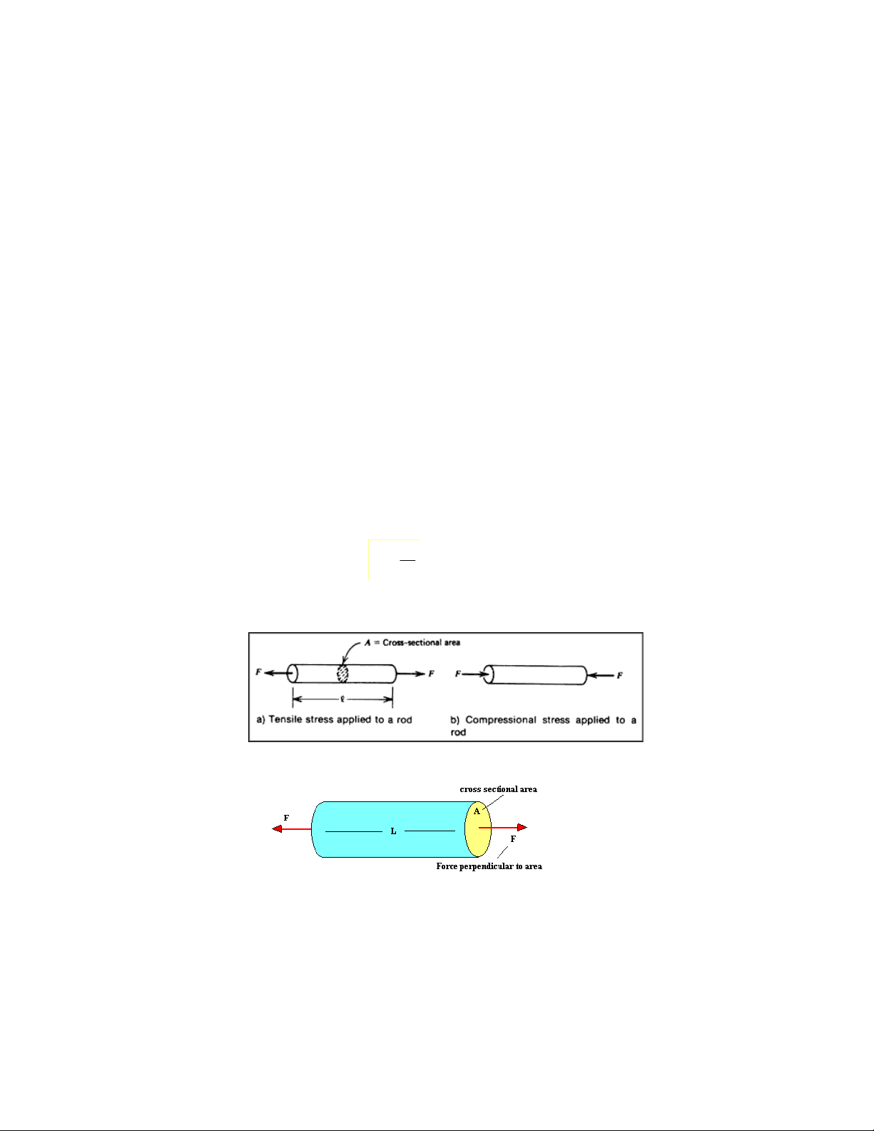
OPTI 521 Kemei Zhao October 11, 2007 Abstract This report first gives the definition of stress and strain, and then gives their relationship in elastic region. The relationship between stress and strain includes uni-axial stress state, pure shear stress state, bi-axial stress state (plane stress), biaxial strain (plane strain) state and tri-axial stress state cases. For uni-axial case, the general stress – strain curve for ductile materials and brittle materials are provided. About ductile materials, some important terms are also introduced. Some definitions Normal stress (axial stress) Normal stress (axial stress) results when a member is subject to an axial load applied through the centric of the cross section. It can be defined in terms of forces applied to a uniform rod [1], numerically it is the ratio of the perpendicular force applied to a specimen divided by its original cross sectional area [2]: A F Figure 1& 2 show the diagram. Normal stress includes tensile and compressive stress, the conventional sign for normal stresses are: tensile stresses are positive (+), compressive stresses are negative (-). The unit of stress is pascals (Pa) (1Pa=1N/m^2 ). Because in practice 1Pa is too small, Mpa, N/mm^2 are usually used. In America, English unit psi (or ksi or Msi) is often used: 1 psi ~= 7000 Pa. Figure 1 Figure 2
Normal strain Normal strain is defined as the ratio of change in length due to deformation to the original length of the specimen [2] : L 0 L Figure 3 shows the diagram. Strain is unitless, but often units of m/m (or mm/mm) are used. In America, inch/inch is often used. Shear stress Shear stress is defined in terms of a couple that tends to deform a joining member (Figure 4) [1]
. It is used in cases where purely sheer force is applied to a specimen, the formula for calculation and units remain the same as tensile stress (Figure 5): A 0 F The unit of shear stress is same as normal stress. Shear strain Figure 3 Figure 4 Figure 5 A 0
As examples, Figure 9, 10, and 11 show s tress-Strain curves of low-carbon steel, Aluminum and glass, respectively [3]. Low-carbon steel and Aluminum belong to ductile material, whereas glass is a kind of typical brittle material. Yield strength is a very important parameter for a material. For any material, yield strength is defined the maximum stress that can be applied without exceeding a specified value of permanent strain (typically 0.2% = .002 in/in). Precision elastic limit or micro- yield strength is another parameter to define the property of a material; it is defined as the maximum stress that can be applied without exceeding a permanent strain of 1 ppm or 0.0001% [3]. For general ductile material, there are two regions in the s tress-Strain curve: elastic region and plastic region (Figure 12). Within the elastic region, there exists a linear relationship between stress and strain, but in plastic region, their relationship is non-linear. Uni-axial Stress State Elastic analysis Figure 13 shows uni-axial stress state: Stresses on inclined planes
Stress Strain Curve
- Similar to Pressure-Volume Curve
- Area = Work Volume Pressure Volume Figure 12 Figure 9 Figure 10 Figure 11 σ σ Figure 13
Stresses on inclined planes (Figure 14) are expressed in following [4]: Stress-strain relationship For materials at relatively low levels, normal stress and strain are proportional through: E The constant E is called Young’s modulus. Thermal strain Strain caused by temperature changes is called thermal strain (Figure 15). It can be calculated by the following formula: α is a material characteristic called the coefficient of thermal expansion. Strain caused by temperature changes and strain caused by applied loads are essentially independent. Therefore, the total amount of strain may be expressed as follows: Figure 14 Figure 15
State of plane stress occurs in a thin plate subjected to forces acting in the mid- plane of the plate. State of plane stress also occurs on the free surface of a structural element or machine component, i.e., at any point of the surface not subjected to an external force (Figure 17). Transformation of stresses Figure 18 schematically shows two elements with angle θ between them. The transformation of stresses between the two planes is [6]: Mohr’s circle for plane stress state Figure 18
Figure 19 is the Mohr’s circle for plane stress state. From the Mohr’s circle, any inclined plane’s stresses can be numerically obtained. For example, the coordinates of the two points H, V are the stresses of an inclined plane with inclined angle θ. The instruction to make the Mohr’s circle is [4]:
- Determine the point on the body in which the principal stresses are to be determined.
- Treating the load cases independently and calculated the stresses for the point chosen.
- Choose a set of x-y reference axes and draw a square element centered on the axes.
- Identify the stresses σx, σy, and τxy = τyx and list them with the proper sign.
- Draw a set of σ - τ coordinate axes with σ being positive to the right and τ being positive in the upward direction. Choose an appropriate scale for the each axis.
- Using the rules on the previous page, plot the stresses on the x face of the element in this coordinate system ( point V ). Repeat the process for the y face ( point H ).
- Draw a line between the two point V and H. The point where this line crosses the σ axis establishes the center of the circle.
- Draw the complete circle.
- The line from the center of the circle to point V identifies the x axis or reference axis for angle measurements ( i.e. θ = 0 ). Note: The angle between the reference axis and the σ axis is equal to 2θp. Principal Stresses and principal planes Figure 19
The angle of the plane where maximum shear stress occurs is: Note: On Mohr’s circle, the planes of maximum shearing stress (points D and E) are at 90^0 to the principal planes (points A and B), but on the element, the planes of maximum shearing stress are at 45^0 to the principal planes. Stress-strain relationship With plane stress assumption, for isotropic material, in elastic region, the stress- strain relationship should be [5]: xy y x xy y x E 2 1 0 0 1 0 1 0 1 2 Note: ( )( ) 1 z x y E Where, E and ν are the Young’s modulus and Poisson’s ratio of the material. (2) Plane strain state For linear, isotropic material, plane stress state assumes that [7]^ (Figure 22): Coordinate Transformation Figure 22
The transformation of strains with respect to the reference { x , y , z } coordinates to the strains with respect to { x' , y' , z' } (Figure 23) is performed via the equations [7]: Mohr’s circle for plane strain state Figure 24 is the Mohr’s circle for plane strain state. The method to construct the circle is similar to that construct Mohr’s circle for plane stress state. Principal Strains and the directions Figure 24 Figure 23
The maximum shear strain is [7]: The angle between the plane that maximum shear strain occurs and reference plane is: Stress-strain relationship With plane stress assumption, for isotropic material, in elastic region, the stress- strain relationship should be [5]:
z y x z y x E
Note: (^) ( ) z 1 1 2 x y E Tri-axial stress state elastic analysis In general, at a point, 3 normal stresses may act on faces of the cube, as well as, 6 components of shear stress (Figure 27). For the 6 shear stresses, only 3 of them are independent, because:
The stain components are shown in Figure 27, too. The stress on an inclined plane To simplify the case, choose a set of reference coordinates (Figure 28) coincident to the principle stresses, and then the stresses σn and τn in any inclined plane with normal direction (l, m, and n) can be calculated by following equtions [9]: ) ( )( ) 2
n^ ^ n l ) ( )( ) 2
n^ ^ n m ) ( )( ) 2
n^ ^ n n Mohr’s circle p
2 y x z (l, m, n)
n
n
Figure 27 Figure 28
[3] Class notes from Dr. J. H. Burge [4] Class notes from Dr. Stone’s OPTI 222 class [5] http://www4.eas.asu.edu/concrete/elasticity2_95/sld001.htm [6] http://www.egr.msu.edu/classes/me423/aloos/lecture_notes/lecture_4.pdf [7] http://www.efunda.com/formulae/solid_mechanics/mat_mechanics/calc_principal_strain.cfm [8] Mechanics of material ( Hongwen Liu ) [9] http://www.shodor.org/~jingersoll/weave4/tutorial/tutorial.html