Download Taylor's Theorem and LaGrange Error Bound: Understanding Function Approximation and Error and more Study notes Design in PDF only on Docsity!
Lesson 4: Taylor’s Theorem &
The LaGrange Error Bound
Where Do We Go From Here
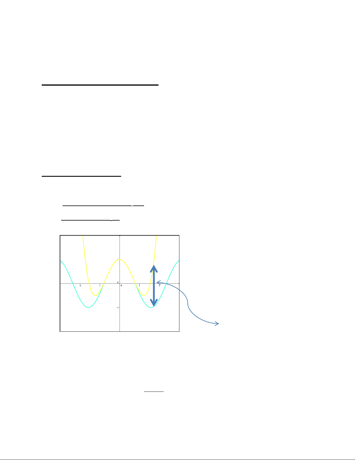
Let’s remember…..we are forming polynomials that approximate functions. So naturally, there is bound to
be some error right?
Our next step is to focus on that error:
Does error matter? How can we find that error?
Does Error Matter?
Every truncation splits a Taylor series into two equally significant pieces:
(a) The Taylor Polynomial Pn(x) - which gives us the approximation
(b) The Remainder Rn(x) - which tells us whether the approximation is any good
Consider the 1986 Challenger disaster…..
Why did that space shuttle crash?
The design of the O-ring was off…..by
th of an inch.
That mistake cost 8 astronauts their lives!
This is the error between the actual function and the polynomial approximation!
Lesson 4: Taylor’s Theorem &
The LaGrange Error Bound
Taylor’s Theorem
If f has derivatives of all orders in an open interval I containing a , then for each positive integer n
and for each x in I ,
The first equation in Taylor’s Theorem is Taylor’s formula. The function Rn(x) is the remainder
of order n or the error term for the approximation of f by Pn(x) over I. It is also called the
Lagrange form of the remainder , and bounds on Rn(x) found using this form are Lagrange
error bounds.
Lagrange Error Bound
OR
In choosing the value for “c”, we should keep in mind that we must maximize this error. This
means that the series approximation to a function value will be AT MOST the value of this error.
We use Taylor polynomials to approximate the values of functions that we cannot evaluate
directly. We are already settling for an approximation. If we could find the exact error in our
approximation, then we would be able to determine the exact value of the function simply by
adding it to the approximation.
( ) 2
( 1) 1
n n n n n n
f a f a
f x f a f a x a x a x a R x
n
where
f c
R x x a
n
for some c between a and x
( 1) ( ) 1 ( ) ( 1)!
n n n
f c R x x a n
1 ( ) ( 1)!
n n
M
R x x a n
Lesson 4: Taylor’s Theorem &
The LaGrange Error Bound
Ex 3:
(a) Find the 3
rd degree Taylor polynomial approximation for ( ) x f x e at x 0.
(b) Use the polynomial to approximate (^) f (1).
(c) Use the Lagrange error bound to prove that the value of f (1)must be less than
0.4.
Ex 4: The approximation
2 ln(1 ) 2
x x x is used when x is small and represents T 2 (^) ( ) x , the
second Taylor polynomial approximation on the interval [ 0.1, 0.1]. Use the Lagrange
error bound to find the maximum error on the approximation of f ( 0.1).
Note that we are given the second order Taylor polynomial, so the remainder must use the third derivative. So we will need to find the third derivative at - 0.1.
Lesson 4: Taylor’s Theorem &
The LaGrange Error Bound
Ex 5 : Use the sixth-order Maclaurin polynomial for the cosine function to approximate cos(2).
Use the Lagrange error bound to give bounds for the value of cos(2). In other words, fill in the blanks:
_____ cos(2) _____
1994 BC4 (parts a and b only) – Calculator Active
Lesson 4: Taylor’s Theorem &
The LaGrange Error Bound
2004 BC6 – We Can DO ALL of it!
No Calculator
Lesson 4: Taylor’s Theorem &
The LaGrange Error Bound
1994 BC4 Answers
2004 (B) BC2 Answers