


CHUANGXINBAN JOURNAL OF COMPUTING, MAR 2018 1
An efficient sorting algorithm — Ultimate
Heapsort(UHS)
Feiyang Chen, Nan Chen, Hanyang Mao, Hanlin Hu
Abstract—Motivated by the development of computer theory, sorting algorithm is emerging in an endless stream. Inspired by decrease
and conquer method, we propose a brand new sorting algorithmUltimately Heapsort. The algorithm consists of two parts: building a
heap and adjusting a heap. Through the asymptotic analysis and experimental analysis of the algorithm, the time complexity of our
algorithm can reach O(nlogn)under any condition.Moreover, its space complexity is only O(1). It can be seen that our algorithm is
superior to all previous algorithms.
Index Terms—Sort algorithm, Min-heap, Max-heap, Asymptotic analysis, Experimental analysis
F
1 INTRODUCTION
SORT ING algorithm is one of the most important re-
search areas in computer science. It has a wide range
of applications in computer graphics, computer-aided de-
sign, robotics, pattern recognition, and statistics. At present,
quicksort is generally considered as the best choice in
practical sorting applications. However, when we need to
dynamically add and delete data during the sorting, we
find that the quicksort can’t exert its performance. There-
fore, we design an efficient sorting algorithm—the ultimate
heapsort(UHS), which offers us a better solution to this type
of problem.
2 ULTI MATE HEAPSORT(UHS)
2.1 Preliminary
We use heap data structure to implement our ultimate
heapsort algorithm. The heap is a complete binary tree, and
it is divided into a max-heap and a min-heap. The max-heap
requires that the value of the parent node is greater than or
equal to the value of the child node, and the min-heap is the
opposite. According to the characteristic of the max-heap,
we can know that the maximum value must be at the top
of the heap, that is, the root node. With this, we can build
an array into a max-heap. Here we take the max-heap as an
example. The min-heap is similar. For our UHS algorithm,
we use max-heaps.
2.2 Main idea
Here we will describe our UHS algorithm’s main idea in
detail. Firstly, we build the array as a max-heap, which is
the initial heap. At this point we know that the top element
of the heap is the maximum, that is, the first element of the
array is the maximum value. Secondly, we swap the first
element of the array with the last one, then the last one will
be the maximum value, and then we update the heap with
the last element removed, ensuring that the first one is at
its maximum in the new heap. Finally, we repeat the above
operation until only one element left.
2.3 Design of the UHS
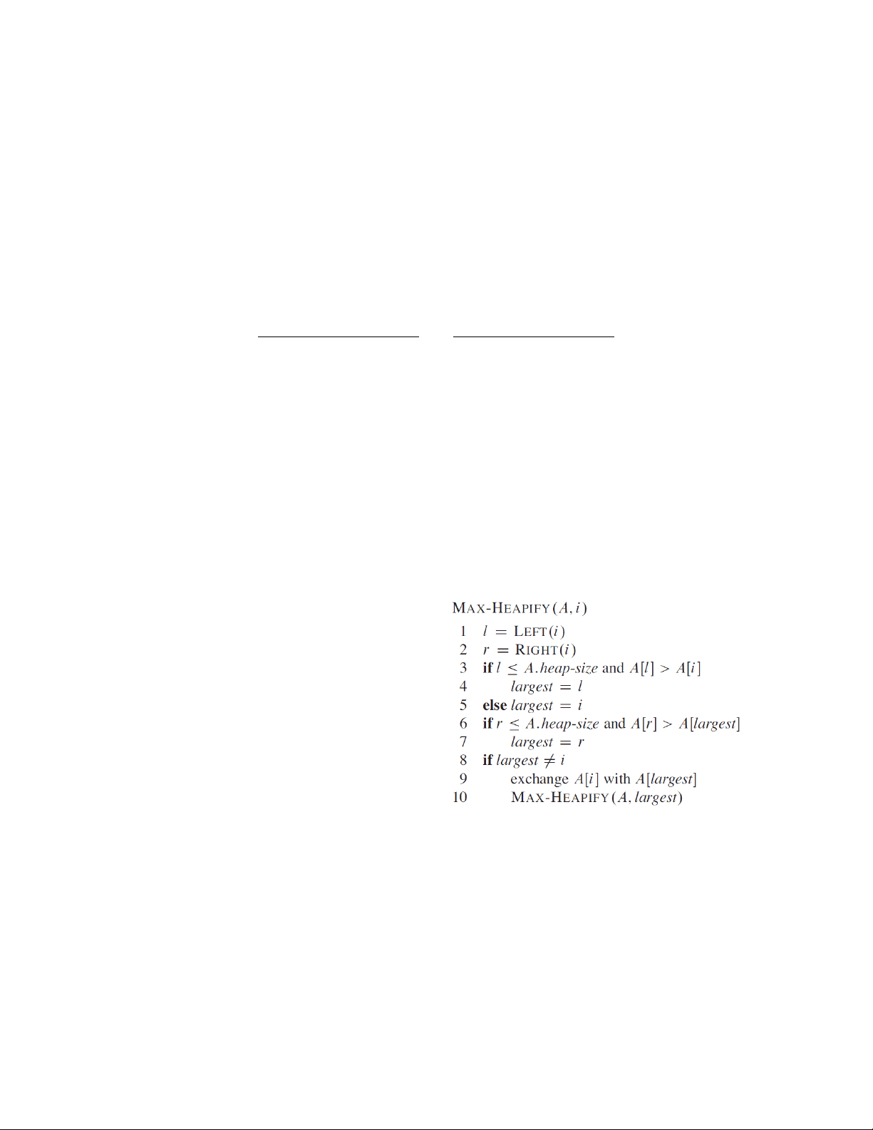
2.3.1 MAX-HEAPLFY
In order to maintain the max-heap property, we call the
procedure MAX-HEAPIFY. Its inputs are an array Aand an
index iinto the array. When it is called, MAX- HEAPIFY
assumes that the binary trees rooted at LEF T (i)and
RIGH T (i)are max- heaps, but that A[i] might be smaller
than its children, thus violating the max-heap property.
MAX-HEAPIFY lets the value at A[i]”float down” in the
max-heap so that the subtree rooted at index iobeys the
max-heap property.
At each step of MAX-HEAPLFY, the largest of the ele-
ments A[i],A[LEF T (i)], and A[RI GHT (i)] is determined,
and its index is stored in largest. IfA[i]is largest, then the
subtree rooted at node iis already a max-heap and the pro-
cedure terminates. Otherwise, one of the two children has
the largest element, and A[i]is swapped with A[largest],
which causes node iand its children to satisfy the max-
heap property. The node indexed by largest, however, now
has the original value A[i], and thus the subtree rooted at
largest might violate the max-heap property. Consequently,
we call MAX-HEAPIFY recursively on that subtree.
2.3.2 Building a heap
We can use the procedure MAX-HEAPIFY in a bottom-up
manner to convert an array A[1..n], where n=A.length,
arXiv:1902.00257v1 [cs.DS] 1 Feb 2019
