Download Analysis of Contingency Tables Contingency Tables ... and more Schemes and Mind Maps Design in PDF only on Docsity!
Psy 525/625 Categorical Data Analysis, Spring 2021 1
Analysis of Contingency Tables Contingency Tables Contingency tables, sometimes called cross-classification or crosstab tables, involve two categorical variables. More generally, we will refer to the two variables as each having I or J levels. For simplicity, we will start by assuming two binary variables, forming a 2 × 2 table, in which I = 2 and J = 2. The four cells of the design can contain counts, nij , or proportions, p (^) ij. The first subscript is an index of which level of the first variable is referred to. In the 2 × 2 case, i = 1 for the first row or i = 2 for the second row, and j = 1 for the first column or j = 2 for the second column. For example, the count in the cell for the intersection of the first column and first row will be n 11. And the count in the cell in the intersection of the first row and second column is n 12 and so on. Marginal values are referred to with a “+” symbol to designate that either i or j have been combined. So, for example, n 1+ is used for the first row marginal total count, and n +1 is used for the first column marginal total count. Cell counts and proportions with the notation are presented below.
Cell counts/frequencies
n 11 n 12 n 1+ n 21 n 22 n 2+ n +1 n +2 n ++
Proportions
p 11 p 12 p 1+ p 21 p 22 p 2+ p +1 p +2 p ++
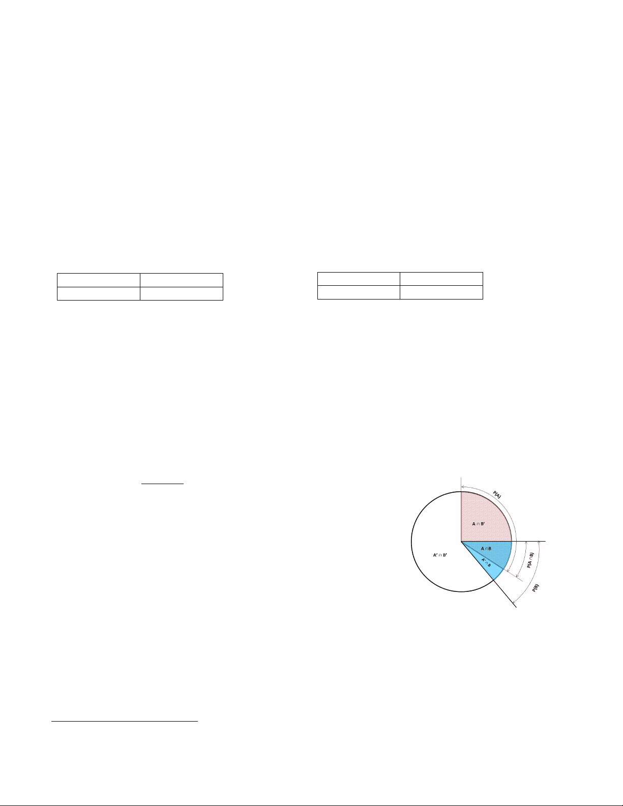
The proportions outside of the cells of each table (e.g., p +1 , p +2 , p 1+, p 2+) are marginal proportions that relate to the marginal distribution for that variable. Each marginal proportion involves only the counts for one of the variables and the total sample size, pi+ = ni + / n ++ and p + j = n + j / n ++. (Note that either n ++ or n may be used). The proportions inside the cells of the table ( p 11 , p 12 , p 21, p 21 ) are joint proportions that relate to the joint distribution of the two variables. Each joint proportion is the count for that cell divided by the total count, pij = nij / n ++. Another distinction is the conditional proportion, which relates to the conditional distribution. Conditional proportions represent estimates of the conditional probability that P ( Y (^) i = 1) given the value of Y (^) j , written as P ( Y (^) i = 1| Y (^) j ).^1 The conditional probability that event A occurs given event B is the same as the joint probability of A and B occurring relative to the probability of B occurring (or the B sample space).
|
P A B P A B P B
∩
Similarly, the sample conditional proportion estimates the conditional probability, such at
pi j (^) | = pij / pi (^) + = nij / ni +
In contingency tables, this is a row proportion (percentage), because it is the proportion of all cases in one row ( ni + ) that appear in one column, nij (e.g., proportion of males that say “no”).
Andrew Batishchev
Bayes’ Theorem It is well worth a brief digression to discuss the famous theorem called Bayes’ theorem , proposed by the eighteenth-century mathematician/clergyman Thomas Bayes, because of its very widespread application to statistics. Bayes’ theorem is a simple method of computing the conditional probability of one event given another event if the probability of both events and the other conditional probability is known.
(^1) The subscripts for the Y variable are potentially confusing, as Y here generally is assumed to be an individual score, with Yi representing the individual score for the row variable with a particular value (e.g., i = 2) and Yj representing the individual score on the column variable with a particular value (e.g., j = 1).
Psy 525/625 Categorical Data Analysis, Spring 2021 2
| |
P B A P A P A B P B
=
In a contingency analysis, we might be interested in computing the probability that an individual who completed a treatment center program will have a drug relapse within six months. If the probability of a relapse in general is .60, the probability of completing a treatment program is .64, and the probability of having completed a program among those who have relapsed before is .3, then the probability that an individual will relapse if he/she has completed the program is approximately .281.
|. .
P B A P A P A B P B
= = =
Bayes’ theorem is the kernel of Bayesian statistics, based upon the notion that informative prior information can be used in this way to better estimate a probability (or other statistic) than just using general information about the distribution. As with the problem above, its utility depends importantly on the accuracy of the prior information.
Conceptualizing Contingency Table Analysis Pearson’s chi-squared test (Pearson, 1900) is easily generalizable to analysis of contingency tables. There are three different but equivalent ways of conceptualizing the test. One is as a test of homogeneity, which refers to whether two groups are different on a binary response (e.g., whether males and females differ in the choice between two candidates). This conceptualization assumes one variable is an explanatory variable and one is a response, but the chi-square does not require such a designation. The goodness-of-fit conceptualization concerns the degree to which the observed frequencies fit the frequencies that would be expected do to chance. The same equation we discussed in the single variable case is also used for contingency analysis, but uses a different set of expected values that take the marginal frequencies of each of the two variables into account.
( )
2 2^ i^ ij , ij
O E E
χ
− = (^) ∑ where each cell’s expected values is^
i j ij
n n E n
++
=
Notice that the expected frequency for each cell is a joint frequency that is expected from the marginal frequencies for each of its respective rows and columns. The larger the discrepancies between the observed and expected frequencies are the greater lack of fit from what is expected due to chance. The third conceptualization is that chi-squared is a test of independence of two binary variables, or, rather, the test of whether they are dependent or correlated. As with correlation, we do not need to designate one variable as an explanatory variable and one as a response under this conceptualization. Although the equation most clearly reflects the goodness-of-fit aspect of the test, it is just as valid to consider it a test of questions about homogeneity or independence.
So, these different interpretations or rationales of chi-square mean that the statistic is useful to test many different types of hypotheses, given a data situation that involves all categorical variables. These three interpretations of chi-square also highlight the fact that when we are testing to see if two groups are different, we are also testing the hypothesis about whether a grouping variable (i.e., the dichotomous independent variable) is correlated with the dependent variable.
Computation Let’s use the Quinnipiac University poll data to examine the extent to which independents (non-party affiliated voters) support Biden and Trump.^2 Here are the frequencies:
(^2) These results are based on a national Quinnipiac University poll from Oct 4-7, 2019, https://poll.qu.edu/national/release- detail?ReleaseID=3643. Methodological details are here https://poll.qu.edu/images/polling/us/us10082019_demos_uljv62.pdf/.
Psy 525/625 Categorical Data Analysis, Spring 2021 4
Pearson chi-square (Agresti, 2003, section 3.2.4). There are a variety of other proposed approaches to the standard error/confidence intervals including a Wald and exact intervals (see Newcombe, 1998).^4
Residuals Residuals, representing the discrepancy between the observed and expected frequencies are sometimes discussed or used in computations of other statistics, and called “Pearson residuals.” The sum of the squared residuals is equal to the Pearson chi-square. Typically, they are standardized by dividing by the standard deviation of the expected proportions, as below.
( 1 ) (^) ( 1 )
ij ij ij ij i j
O E r E p (^) + p +
−
− −
For the standardized Pearson residuals, each cell can be evaluated for difference from what is expected under the null hypothesis using the z distribution or the chi-squared distribution, because r (^) ij = z (^) ij and 2 2 r ij = χ ij.
Minimum Expected Frequencies and Fisher’s Exact Test Fisher’s exact test, proposed by R.A. Fisher (Fisher, 1935) and sometimes called the “Fisher-Irwin” test,
is often printed along with the Pearson χ^2. It is not so much a modification of the chi-square test as an
alternative approach to testing the association between two binary variables for significance. The test has been suggested for use with small samples in which the expected frequencies in some cells are low. The concept is to use the hypergeometric distribution to compute the exact probability of the particular configuration of obtained frequencies. If the marginal frequencies ( n +1 and n 1+) that related to one of the cells, say n 11 , remain the same, the Fisher’s exact test asks how likely the obtained frequency is compared to all of the other more or less extreme outcomes. Only one cell is needed because the other cell counts are determined given a certain count in n 11 as long as the marginal frequencies are the same. The hypergeometric distribution function bears some resemblance to the binomial distribution function which was based on combinatorials for probability of all the possible outcomes. The probability of occurrence of any given obtained frequency for n 11 given its marginal frequencies is P ( n 11 ).
11 12 21 22 11 21 11 12 21 22 11 21 21 22 11 11 12 21 22 11 21
!!!! !!!!!
n n n n n n n n n n n n n n P n n (^) n n n n n n n
++ ++
+^ + (^) + + + + = ^ ^ = (^) +
The estimated probability is then compared to probabilities for other configurations of possible cell frequencies given the same marginal frequencies, but with more extreme results. If n +1 and n 1+ are both 12, the possible values between the null and most extreme alternative hypothesis range from 6 to12. Fisher used the approach in the famous test of his colleague Dr. Muriel Bristol’s assertion that she could taste the difference between cups of tea in which the milk was added first compared with cups in which the milk was added last.^5 The test was originally a one-tailed test and Irwin (1935) proposed a two-tailed approach. The problem with Fisher’ exact test is that it can be overly conservative and its use is often recommended when not necessary. Some software packages print a warning when 20% of the cells have an expected frequency below 5 (known as Cochran’s rule). First thing to notice, however, is that it is the expected frequency that is of concern and not the observed frequency. Secondly, simulation
studies (e.g., Camilli & Hopkins, 1978) suggest that Pearson’s χ^2 has nominal alpha values with
(^4) The Wald SE is 1 (^1 )^2 (^2 ) 1 2
p 1 p p 1 p n n
− (^) + −. See Caffo (2007) http://ocw.jhsph.edu/courses/MethodsInBiostatisticsII/PDFs/lecture18.pdf.
(^5) Incidentally, if you are a complete stat geek like me, you will enjoy David Salsburg’s book The Lady Tasting Tea: How Statistics Revolutionized Science in the Twentieth Century.
Psy 525/625 Categorical Data Analysis, Spring 2021 5
expected values as low as 1 as long as the total sample size is 20 or larger. So, the upshot is that Fisher’s exact test is not needed in very many circumstances. Yates’ Continuity Correction
Yates suggested a correction to the Pearson’s χ^2 based on the notion that a test of discrete variables
which should follow a discrete distribution are tested using a normal approximation, the chi-squared distribution. The Yates’ correction for continuity is a simple modification of the chi-squared test formula by subtracting ½ or .5 from the frequency difference.
2 2 i^ ij. ij
O E E
χ
− −
There is good evidence and fairly wide consensus that the results with the Yates correction are too conservative (e.g., Grizzle, 1967; Camilli & Hopkins, 1978).
Partitioning The chi-squared values for the set of all possible orthogonal chi-squares add up to the chi-square for the whole design (or the omnibus test). The likelihood ratio test, G^2 , however, cannot be partitioned in the
same way. Planned follow-up analyses to an omnibus Pearson χ^2 in complex contingency tables are
simply chi-square analyses based on chi-squared tests for two-cell comparisons or smaller contingency tables (e.g., a 2 × 2 from a 5 × 3 design). Such tests may involve marginal proportions or cell proportions as well. With many post hoc tests, the researcher may wish to use a familywise error adjustment. The straight Bonferroni, although the most commonly applied, is overly conservative. I recommend other alternatives instead (e.g., Hochberg’s sequential or Sidák-Bonferroni). General procedures for any set of significance tests in SAS (PROC MULTEST) and R (p.adjust) can provide some of these tests.
Comparing Chi-squared Values It is also possible to compare two independent (between subjects not repeated measures) chi-squared values. The formula below (D’Agostino & Rosman, 1971) assumes the same dimensional tables and, therefore, the same df.
2 2 1 2
1 1 4
z df
χ − χ
− ^
Three or More Dimensions Although 2 × 2 contingency table looks like a 2 × 2 factorial table, they are not analogous. The homogeneity conceptualization of chi-squared tests involves a two-group comparison of a binary outcome, which is analogous to a t -test in the continuous case. Because one of the columns (or rows) is for the dependent variable, it is really the three-way table that is analogous to the factorial design in ANOVA, which requires an analysis of a three-way contingency table (2 × 2 × 2) in the binary outcome case. I will cover these tests in the next section.
Software Examples
Below I illustrate SPSS, R, and SAS procedures for the Pearson’s χ^2 test to independents on their
favorability of the two candidates using the Reuters polling data.
SPSS The crosstabs table has row (% within ind), column (% within response), and total (% of total) percents, although I usually only request percent row (or column) in practice.
SPSS
Psy 525/625 Categorical Data Analysis, Spring 2021 7
Sum 1.000 1.
To get marginal frequencies and proportions in R > BarChart (response, by=ind, horiz = FALSE, stat = "proportion", beside = TRUE)
Joint and Marginal Frequencies
response ind 0 1 Sum 0 338 363 701 1 125 156 281 Sum 463 519 982
Cramer's V (phi): 0.
Chi-square Test: Chisq = 1.122, df = 1, p-value = 0.
Cell Proportions within Each Column
response ind 0 1 0 0.730 0. 1 0.270 0. Sum 1.000 1.
> # the MASS package also can be used > library(MASS) > tbl = table(d$ind, d$response) > tbl
0 1 0 338 363 1 125 156 > > margin.table(tbl, 2) # Frequencies summed over ind
0 1 463 519 > > chisq.test(tbl,correct = FALSE) #correct = FALSE turns off Yates continuity correction
Pearson's Chi-squared test
data: tbl X-squared = 1.1217, df = 1, p-value = 0.
Psy 525/625 Categorical Data Analysis, Spring 2021 8
SAS contingency chi-square; proc freq data=one; tables indresponse /chisq; run ;
ind(ind vs affil) response(intended vote)
Frequency ‚ Percent ‚ Row Pct ‚ Col Pct ‚Trump ‚Biden ‚ Total ƒƒƒƒƒƒƒƒƒƒƒƒˆƒƒƒƒƒƒƒƒˆƒƒƒƒƒƒƒƒˆ affiliate ‚ 338 ‚ 363 ‚ 701 ‚ 34.42 ‚ 36.97 ‚ 71. ‚ 48.22 ‚ 51.78 ‚ ‚ 73.00 ‚ 69.94 ‚ ƒƒƒƒƒƒƒƒƒƒƒƒˆƒƒƒƒƒƒƒƒˆƒƒƒƒƒƒƒƒˆ independent ‚ 125 ‚ 156 ‚ 281 ‚ 12.73 ‚ 15.89 ‚ 28. ‚ 44.48 ‚ 55.52 ‚ ‚ 27.00 ‚ 30.06 ‚ ƒƒƒƒƒƒƒƒƒƒƒƒˆƒƒƒƒƒƒƒƒˆƒƒƒƒƒƒƒƒˆ Total 463 519 982 47.15 52.85 100.
Frequency Missing = 6
Statistics for Table of ind by response
Statistic DF Value Prob ƒƒƒƒƒƒƒƒƒƒƒƒƒƒƒƒƒƒƒƒƒƒƒƒƒƒƒƒƒƒƒƒƒƒƒƒƒƒƒƒƒƒƒƒƒƒƒƒƒƒƒƒƒƒ Chi-Square 1 1.1217 0. Likelihood Ratio Chi-Square 1 1.1235 0. Continuity Adj. Chi-Square 1 0.9769 0. Mantel-Haenszel Chi-Square 1 1.1205 0. Phi Coefficient 0. Contingency Coefficient 0. Cramer's V 0.
Fisher's Exact Test ƒƒƒƒƒƒƒƒƒƒƒƒƒƒƒƒƒƒƒƒƒƒƒƒƒƒƒƒƒƒƒƒƒƒ Cell (1,1) Frequency (F) 338 Left-sided Pr <= F 0. Right-sided Pr >= F 0.
Table Probability (P) 0. Two-sided Pr <= P 0.
Sample Size = 982 Frequency Missing = 6
Example write-up. A chi-square test was used to determine whether there was a significant difference between the proportion of Biden and Trump's supporters who are independent. Results indicated that 30.1% of Biden's supporters were independents, whereas 27.0% of Trumps supporters were
independents. This difference was not significant, χ^2 (1) = 1.12, p = .29 The phi coefficient, φ = .03,
suggested a small effect.