Download Global Optimization: Lecture 16 - Global Dataflow Analysis and Constant Propagation and more Study notes Computer Science in PDF only on Docsity!
Prof. Su ECS 142 Lecture 16 1
Global Optimization
ECS 142
Prof. Su ECS 142 Lecture 16 2
Lecture Outline
- Global dataflow analysis
- Two example dataflow analyses
- Global constant propagation
- Liveness analysis
Prof. Su ECS 142 Lecture 16 3
Local Optimization
Recall the simple basic-block optimizations
- Constant propagation
- Dead code elimination
X := 3 Y := Z * W Q := X + Y
X := 3 Y := Z * W Q := 3 + Y
Y := Z * W Q := 3 + Y
Prof. Su ECS 142 Lecture 16 4
Global Optimization
These optimizations can be extended to an entire control-flow graph X := 3 B > 0
Y := Z + W Y := 0
A := 2 * X
Prof. Su ECS 142 Lecture 16 5
Global Optimization
These optimizations can be extended to an entire control-flow graph X := 3 B > 0
Y := Z + W Y := 0
A := 2 * X
Prof. Su ECS 142 Lecture 16 6
Global Optimization
These optimizations can be extended to an entire control-flow graph X := 3 B > 0
Y := Z + W Y := 0
A := 2 * 3
Prof. Su ECS 142 Lecture 16 7
Correctness
- How do we know it is OK to globally propagate constants?
- There are situations where it is incorrect:
X := 3 B > 0
Y := Z + W X := 4
Y := 0
A := 2 * X Prof. Su ECS 142 Lecture 16 8
Correctness (Cont.)
To replace a use of x by a constant k we must know that:
On every path to the use of x, the last assignment to x is x := k **
Prof. Su ECS 142 Lecture 16 9
Example 1 Revisited
X := 3 B > 0
Y := Z + W Y := 0
A := 2 * X
Prof. Su ECS 142 Lecture 16 10
Example 2 Revisited
X := 3 B > 0
Y := Z + W X := 4
Y := 0
A := 2 * X
Prof. Su ECS 142 Lecture 16 11
Discussion
- The correctness condition is not trivial to check
- “All paths” includes paths around loops and through branches of conditionals
- Checking the condition requires global analysis
- An analysis of the entire control-flow graph
Prof. Su ECS 142 Lecture 16 12
Global Analysis
Global optimization tasks share several traits:
- The optimization depends on knowing a property X at a particular point in program execution
- Proving X at any point requires knowledge of the entire method body
- It is OK to be conservative. If the optimization requires X to be true, then want to know either - X is definitely true - Don’t know if X is true
- It is always safe to say “don’t know”
Prof. Su ECS 142 Lecture 16 19
Explanation
- The idea is to “push” or “transfer” information from one statement to the next
- For each statement s, we compute information about the value of x immediately before and after s C (^) in(x,s) = value of x before s C (^) out(x,s) = value of x after s
Prof. Su ECS 142 Lecture 16 20
Transfer Functions
- Define a transfer function that transfers information one statement to another
- In the following rules, let statement s have immediate predecessor statements p 1 ,…,pn
Prof. Su ECS 142 Lecture 16 21
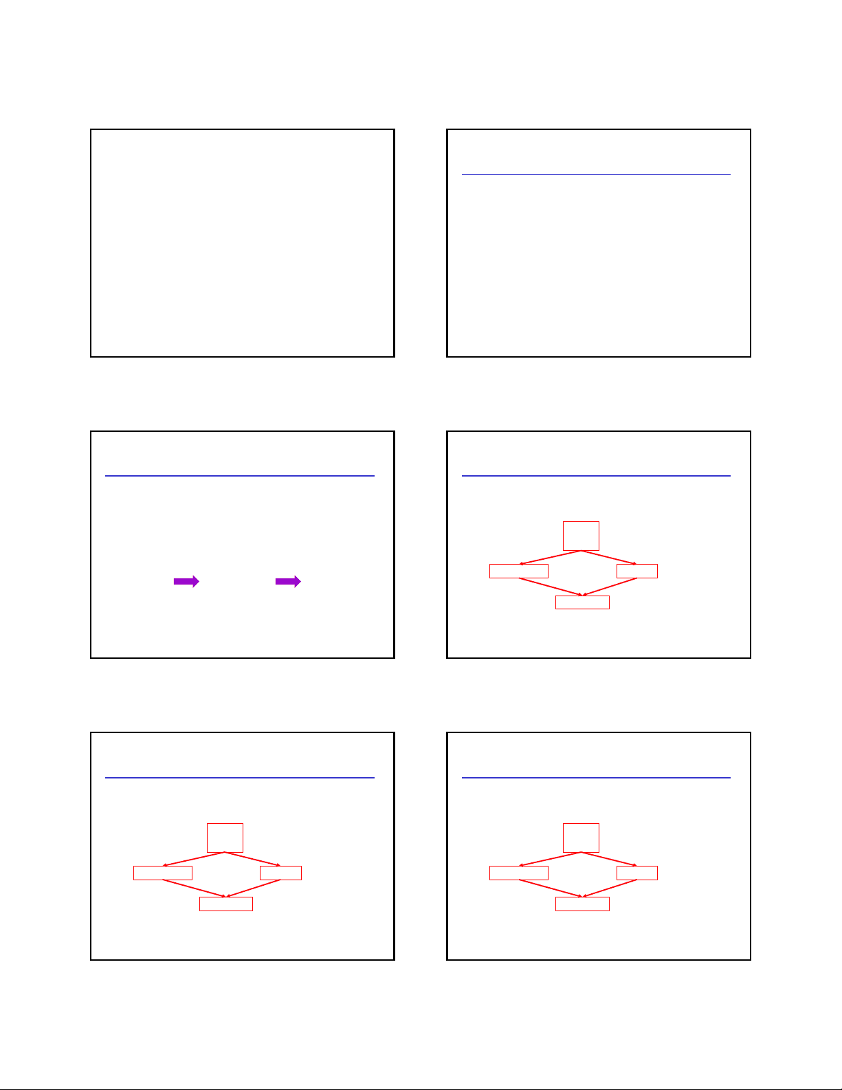
Rule 1
if C (^) out(x, pi) = * for some i, then C (^) in(x, s) = *
s
X = *
X = *
X =? X =? X =?
Prof. Su ECS 142 Lecture 16 22
Rule 2
If C (^) out(x, pi) = c and C (^) out(x, p (^) j) = d and d ≠ c then C (^) in (x, s) = *
s
X = d
X = *
X = c X =? X =?
Prof. Su ECS 142 Lecture 16 23
Rule 3
if C (^) out(x, pi) = c or # for all i, then C (^) in(x, s) = c
s
X = c
X = c
X = c X = # X = #
Prof. Su ECS 142 Lecture 16 24
Rule 4
if C (^) out(x, pi) = # for all i, then C (^) in(x, s) = #
s
X = #
X = #
X = # X = # X = #
Prof. Su ECS 142 Lecture 16 25
The Other Half
- Rules 1-4 relate theout of one statement to thein of the successor statement - they propagate information forward across a CFG edge
- Now we need rules relating thein of a statement to theout of the same statement - to propagate information across statements
Prof. Su ECS 142 Lecture 16 26
Rule 5
C (^) out(x, s) = # if C (^) in(x, s) = #
s
X = #
X = #
Prof. Su ECS 142 Lecture 16 27
Rule 6
C (^) out(x, x := c) = c if c is a constant
x := c
X =?
X = c
Prof. Su ECS 142 Lecture 16 28
Rule 7
C (^) out(x, x := f(…)) = *
x := f(…)
X =?
X = *
Prof. Su ECS 142 Lecture 16 29
Rule 8
C (^) out(x, y := …) = C (^) in(x, y := …) if x ≠ y
y :=...
X = a
X = a
Prof. Su ECS 142 Lecture 16 30
An Algorithm
- For every entry s to the program, set C (^) in(x, s) = *
- Set C (^) in(x, s) = C (^) out(x, s) = # everywhere else
- Repeat until all points satisfy 1-8: Pick s not satisfying 1-8 and update using the appropriate rule
Prof. Su ECS 142 Lecture 16 37
Example
X := 3 B > 0
Y := Z + W Y := 0
A := 2 * X A < B
X = * X = 3
X = 3
X = 3
X = 3
X = 3 X = 3
X = 3
Prof. Su ECS 142 Lecture 16 38
Orderings
- We can simplify the presentation of the analysis by ordering the values # < c < *
- Drawing a picture with “lower” values drawn lower, we get
… -1 0 1 …
Prof. Su ECS 142 Lecture 16 39
Orderings (Cont.)
- is the greatest value, # is the least
- All constants are in between and incomparable
- Letlub be the least-upper bound in this ordering
- Rules 1-4 can be written using lub: Cin(x, s) = lub { Cout(x, p) | p is a predecessor of s }
Prof. Su ECS 142 Lecture 16 40
Termination
- Simply saying “repeat until nothing changes” doesn’t guarantee that eventually nothing changes
- The use of lub explains why the algorithm terminates - Values start as # and onlyincrease - # can change to a constant, and a constant to * - Thus, C_(x, s) can change at most twice
Prof. Su ECS 142 Lecture 16 41
Termination (Cont.)
Thus the algorithm is linear in program size
Number of steps =
Number of C_(….) values computed * 2 =
Number of program statements * 4
Prof. Su ECS 142 Lecture 16 42
Liveness Analysis
Once constants have been globally propagated, we would like to eliminate dead code
After constant propagation, X := 3 is dead (assuming X not used elsewhere)
X := 3 B > 0
Y := Z + W Y := 0
A := 2 * X
Prof. Su ECS 142 Lecture 16 43
Live and Dead
- The first value of x is dead (never used)
- The second value of x is live (may be used)
- Liveness is an important concept
X := 3
X := 4
Y := X
Prof. Su ECS 142 Lecture 16 44
Liveness
A variable x is live at statement s if
- There exists a statement s’ that uses x
- There is a path from s to s’
- That path has no intervening assignment to x
Prof. Su ECS 142 Lecture 16 45
Global Dead Code Elimination
- A statement x := … is dead code if x is dead after the assignment
- Dead statements can be deleted from the program
- But we need liveness information first...
Prof. Su ECS 142 Lecture 16 46
Computing Liveness
- We can express liveness in terms of information transferred between adjacent statements, just as in copy propagation
- Liveness is simpler than constant propagation, since it is a boolean property (true or false)
Prof. Su ECS 142 Lecture 16 47
Liveness Rule 1
Lout(x, p) = ∨ { Lin(x, s) | s a successor of p }
p
X = true
X = true
X =? X =? X =?
Prof. Su ECS 142 Lecture 16 48
Liveness Rule 2
Lin(x, s) = true if s refers to x on the rhs
…:= f(x)
X = true
X =?