Download In-Place Stable Sorting Algorithms and Lower Bounds and more Study notes Digital Systems Design in PDF only on Docsity!
Lecture No.
4.4 In-place, Stable Sorting
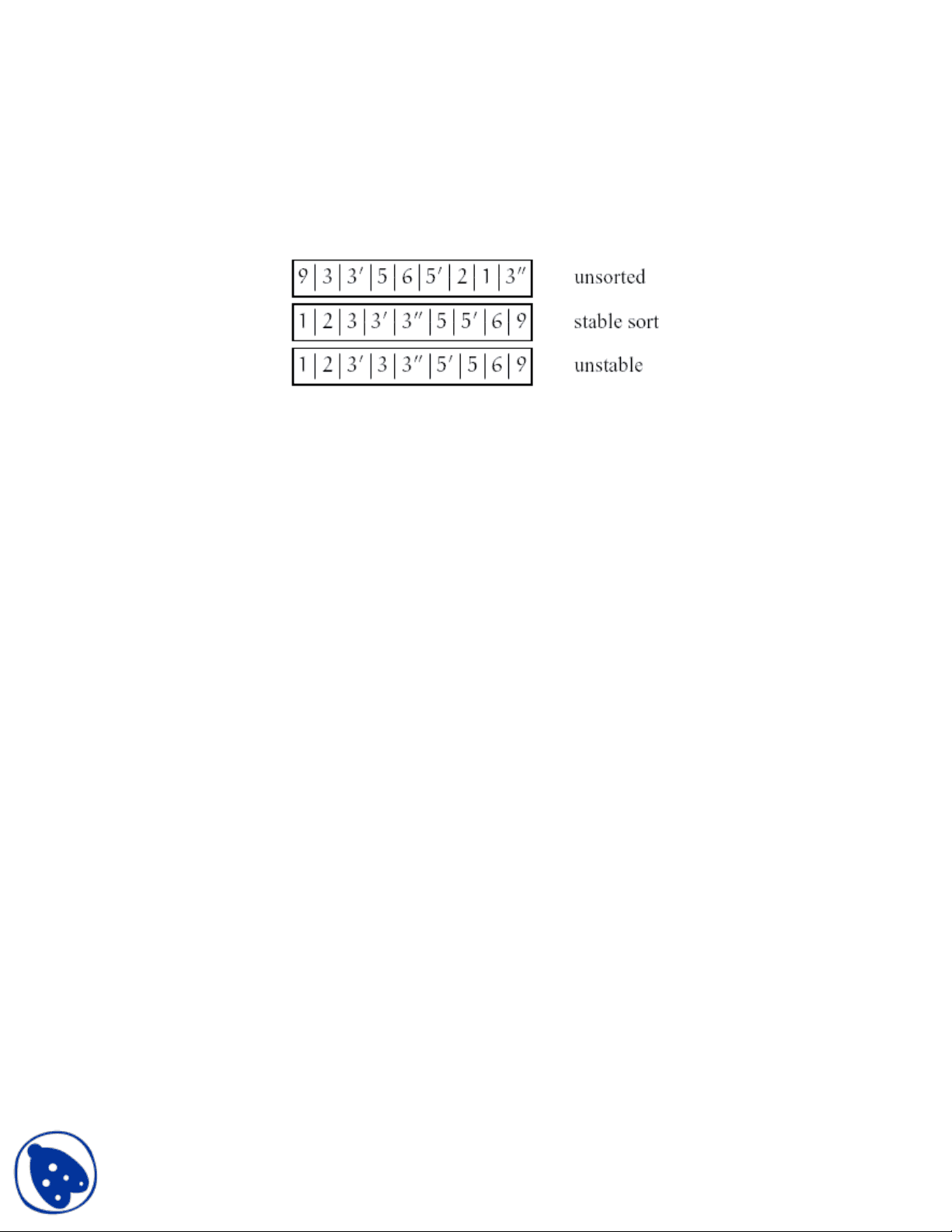
An in-place sorting algorithm is one that uses no additional array for storage. A sorting algorithm is stable if duplicate elements remain in the same relative position after sorting.
Bubble sort, insertion sort and selection sort are in-place sorting algorithms. Bubble sort and insertion sort can be implemented as stable algorithms but selection sort cannot (without significant modifications). Mergesort is a stable algorithm but not an in-place algorithm. It requires extra array storage. Quicksort is not stable but is an in-place algorithm. Heapsort is an in-place algorithm but is not stable.
4.5 Lower Bounds for Sorting
The best we have seen so far is O(n log n) algorithms for sorting. Is it possible to do better than O(n log n)? If a sorting algorithm is solely based on comparison of keys in the array then it is impossible to sort more efficiently than (n log n) time. All algorithms we have seen so far are comparison-based sorting algorithms. Consider sorting three numbers a 1 , a 2 , a 3. There are 3! = 6 possible combinations:
(a 1 , a 2 , a 3 ), (a 1 , a 3 , a 2 ) , (a 3 , a 2 , a 1 ) (a 3 , a 1 , a 2 ), (a 2 , a 1 , a 3 ) , (a 2 , a 3 , a 1 )
One of these permutations leads to the numbers in sorted order. The comparison based algorithm defines a decision tree. Here is the tree for the three numbers. 2 3, 1, 2
1,
2 Figure 4.7: Decision Tree For n elements, there will be n! possible permutations. The height of the tree is exactly equal to T(n), the running time of the algorithm. The height is T(n) because any path from the root to a leaf corresponds to a sequence of comparisons made by the algorithm. Any binary tree of height T(n) has at most 2 T(n) leaves. Thus a comparison based sorting algorithm can distinguish between at most 2 T(n) different final outcomes. So we have
2 T(n) _ n! and therefore T(n) ≥ log(n!)
We can use Stirling’s approximation for n!:
n! √ 2 πn(n/e)n
Thereofore
T(n) ≥ log ( √ 2 πn (n/e)n^ )
= log ( √ 2 πn + n log n – n log e )
= ∈ Ω (n log n) We thus have the following theorem.
Theorem 1 Any comparison-based sorting algorithm has worst-case running time(n log n).
There are four (unnested) loops, executed k times, n times, k - 1 times, and n times, respectively, so the total running time is Θ(n + k) time. If k = O(n), then the total running time is Θ(n). Figure 5.1 through 5.19 shows an example of the algorithm. You should trace through the example to convince yourself how it works. 7
1 2 3 4 5 6 7 8 9 10 11 Figure 5.1: Initial A and C arrays.
7 1 3 1 2 4 5 n ]
Figure 5.2: A[1] = 7 processed 7
Figure 5.3: A[2] = 1 processed 7 1 3 1 2 4 5 7 2 4 ]
Figure 5.4: A[3] = 3 processed
Figure 5.5: A[4] = 1 processed
Figure 5.6: A[5] = 2 processed ]
Figure 5.9: A[11] placed in output array B 11 2 4 5 8
Figure 5.10: A[10] placed in output array B 7 2
Figure 5.11: A[9] placed in output array B
11
Figure 5.12: A[8] placed in output array B
1 Figure 5.15: A[5] placed in output array B
1 10 9 8 6 5 2 C
Figure 5.16: A[4] placed in output array B
10 1 2 5 7 8 9 C
Figure 5.17: A[3] placed in output array B 10 1 2 4 7 8 9 C 1 2 3 4 5 6 7
Figure 5.18: A[2] placed in output array B 10 0 2 4 7 8 9 C 1 2 3 4 5 6 7
Figure 5.20: Stability of counting sort
5.2 Bucket or Bin Sort Assume that the keys of the items that we wish to sort lie in a small fixed range and that there is only one item with each value of the key. Then we can sort with the following procedure:
1. Set up an array of “bins” - one for each value of the key - in order, 2. Examine each item and use the value of the key to place it in the appropriate bin.
Now our collection is sorted and it only took n operations, so this is an O(n) operation. However, note that it will only work under very restricted conditions. To understand these restrictions, let’s be a little more precise about the specification of the problem and assume that there are m values of the key. To recover our sorted collection, we need to examine each bin. This adds a third step to the algorithm above,
3. Examine each bin to see whether there’s an item in it.
which requires m operations. So the algorithm’s time becomes:
T(n) = c 1 n + c 2 m and it is strictly O(n +m). If m _ n, this is clearly O(n). However if m >> n, then it is O(m). An implementation of bin sort might look like:
B UCEKT S ORT( array A, int n, int M)
1 // Pre-condition: for 1 < i ≤ n, 0 ≤ a[i] < M 2 // Mark all the bins empty 3 for i ← 1 to M 4 do bin[i] ← Empty 5 for i ← 1 to n 6 do bin[A[i]] ← Α[i]
If there are duplicates , then each bin can be replaced by a linked list. The third step then becomes:
3. Link all the lists into one list.
.68 Figure 5.22: Bucket sort: step 2, concatenate the lists
Figure 5.23: Bucket sort: the final sorted sequence