Objective of Image Enhancement-Digital Image Processing-Lecture Slides, Slides of Digital Image Processing

Download Objective of Image Enhancement-Digital Image Processing-Lecture Slides and more Slides Digital Image Processing in PDF only on Docsity!

5

Types of image enhancementoperations 

Point/Pixel operationsOutput

value

at

specific

coordinates

(x,y) is dependent only on the inputvalue at (x,y)



Local operationsThe output value at (x,y) is dependenton

the

input

values

in

the

neighborhood of (x,y)



Global operationsThe output value at (x,y) is dependenton all the values in the input image

6

Basic concepts Spatial

domain

enhancement

methods

can

be

generalized

as

g(x,y)=T[f(x,y)]

f(x,y): input imageg(x,y): processed (output) imageT[*]:

an operator on f (or a set of input

images), defined over neighborhood of (x,y)

8

Basic concepts

g(x,y) = T [f(x,y)]



Pixel/point operation:



Neighborhood of size 1x1: g depends only on f at (x,y)



T: a gray-level/intensity transformation/mapping function



Let r = f(x,y) & s = g(x,y), (r and s represent gray levelsof f and g at (x,y)), then

s = T(r)



Local operations:



g depends on the predefined number of neighbors of f at(x,y)



Implemented by using mask processing or filtering



Masks (filters, windows, kernels, templates): a small (e.g.3×3) 2-D array, in which the values of the coefficientsdetermine the nature of the process

9

Basic gray level transformations 

Image negatives



Log transformations



Power-lawtransformations

11

Image scaling

S = T(r) = a.r

(‘a’ is a constant)

12

Log transformations

s = T(r) = c.log(1+r)

14

Log transformations

Fourier spectrum: image values

ranging from 0 to 1.5x

6

Scaled linearly for display purpose

The result of log transformation

with c = 1

15

Power-law transformationsS = T(r) = c.r



c and

are positive

17

Power-law transformation:Gamma Correction 

Gamma correction



To make the CRT response linear, a pre-distortioncircuit is needed

s = cr

1/



18

Power-law transformation:Gamma Correction

20

Power-law transformation:Contrast enhancement

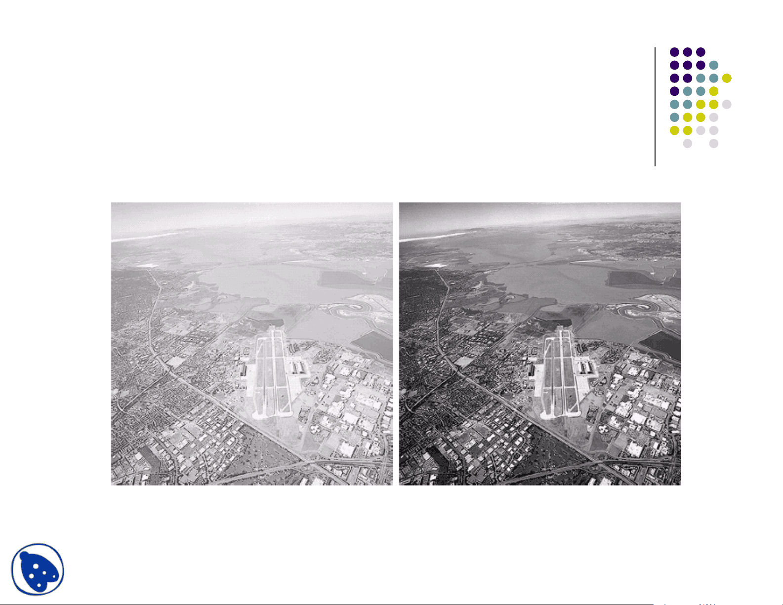
Aerial Image

Result ofPower lawtransformationc = 1,



= 3.

(suitable)

Result of

Power law

transformation

c = 1,



= 4.

(suitable)

Result ofPower lawtransformationc = 1,



= 5.

(high contrast,some regions aretoo dark, somedetails are lost)

21

Piecewise-lineartransformation function

Examples: Contrast stretch, Gray level slicing, etc.Contrast stretch 

Objective:

Increase the dynamic range of the gray

levels for low contrast images



Low contrast images can result from: 

poor illumination



lack of dynamic range in the imaging sensor



wrong setting of a lens aperture during image acquisition