Download Priority Queues and Heaps and more Exams Computer Programming in PDF only on Docsity!
601.433/633 Introduction to Algorithms Lecturer: Michael Dinitz Topic: Priority Queues / Heaps Date: 9/27/
8.1 Introduction
In this lecture we’ll talk about a useful abstraction, priority queues, which are usually implemented through data structures known as heaps. In fact, priority queues are so closely identified with heaps that the terms are sometimes used interchangeably.
In a normal queue we insert elements (known as a push) and remove elements (known as a pop). Because it’s a queue, pops happen in first-in-first-out (FIFO) order. This means that the obvious data structure is a linked list. In a priority queue, the order of pops is by priority, rather than in FIFO order. That is, we think of inserting elements which have keys which have a total order – for concreteness, let’s set all keys to be integers. And since we don’t actually care about the data in the elements, we’ll just think of inserting integers. Then the intuition is that we should always pop off the smallest remaining key, no matter when it was inserted.
Slightly more formally, we want to support the following operations^1 :
- Insert(H, x): insert element x into the heap H
- Extract-Min(H): remove and return an element with smallest key
- Decrease-Key(H, x, k): decrease the key of x to k.
- Meld(H 1 , H 2 ): replace heaps H 1 and H 2 with their union
The following operations are also sometimes useful:
- Find-Min(H): return the element with smallest key
- Delete(H, x): delete element x from heap H
What if we try to do this with just a linked list? Insert is O(1), Meld is O(1), and depending on exactly how its implemented (if we assume the user has pointers to individual elements) Insert and Decrease-Key might take O(1) time. But what about Extract-Min? We would need to look through the entire list, so we only get a running time bound of O(n). Similarly, keeping a sorted linked list or array would make Insert take O(n) time.
Another option would be to use a balanced search tree (e.g., a B-tree or a red-black tree). In this case it’s easy to see that Insert, Find-Min, and Extract-Min all take O(log n) time. It’s not quite as trivial, but it’s not too hard to see that we can also do Delete and Decrease-Key in O(log n) time.
(^1) The element x in these operations is actually a pointer to the actual key – since we are not necessarily getting a lookup operation (like in search trees), we cannot efficiently find a key in the heap, so we assume that we actually have a pointer to it if we want to modify it.
However, the obvious way to Meld would be to just remove the elements one at a time from one tree and add them into the other, giving a cost of O(n log n). We can do a slightly more efficient version of Meld in this case (getting it down to O(n)), but it’s still pretty inefficient.
Note that it’s clearly impossible to make Insert O(1) and Extract-Min O(1), since that would imply an O(n)-time sorting algorithm in the comparison model. But we can hopefully make one of them O(1) and make the other O(log n).
It turns out that heaps can be made extremely efficient. We’re going to try to get some (though not all) of these operations down to constants. The best known bounds are for a structure known as strict Fibonacci heaps, but we won’t have time to discuss them in detail. Instead, we’ll first discuss binary heaps, and then an improvement known as binomial heaps. Note: binary heaps are in the textbook, as are Fibonacci heaps, but binomial heaps aren’t. I think that Fibonacci heaps are a bit too complicated/technical for this class, and that binomial heaps contain many (though not all) of the important ideas, so I’m going to discuss the simpler binomial setting. I’ve added some non-book resources to the course webpage on binomial heaps, and if you’re interested you can also check out the book chapter on Fibonacci heaps.
8.2 Aside: amortized analysis of multiple operations
In last class, we said that the amortized cost of a series of m operations is the total cost of all of them divided by m. But in this class we’re going to make statements about different operations, e.g., “the amortized time for Insert is O(1) and the amortized time for Extract-Min is O(log n).” What does this mean? Well, we just need to generalize to multiple types of operations. If we have k different types of operations, and we prove that the amortized cost of operation type i is αi, then this means that the total cost of any sequence which performs mi operations of type i is
∑k i=1 miαi. This is the obvious generalization of our definition from last time. These kinds of guarantees make it much harder to prove anything directly about the total cost of the sequence, so we will almost always use accounting or potential arguments.
8.3 Binary Heaps
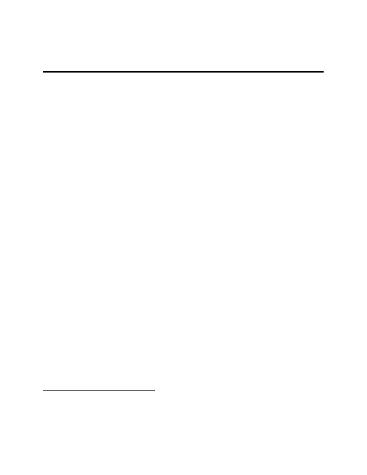
A binary heap is essentially just a complete binary tree, where the only nodes that can be missing are on the bottom level. We make sure that at the bottom level, nodes are filled in from “left” to “right”. The only additional requirement is that the nodes are in heap order : the key of any node is no larger than the key of its children. So as we move up the tree keys are non-increasing, but in different branches the keys are not particularly related. Note that heap order implies that the minimum node is at the root, since if it were anywhere else it would have a parent which was larger than it.
Note that since binary heaps are essentially complete binary trees, we know that their height is at most log n. This is a great property to have, since often the running time of an operation will depend on the height.
Let’s see an example heap:
12 18 11 25
21 17 19 7
8
12 10 11 25
21 17 19
7
6
18
add key to heap (violates heap order)
swim up
- Extract-Min(H): we know because of heap ordering that the minimum as at the root. So Find-Min(H) is easy: simply return the root, which takes O(1) time. But to do Extract-Min we need to also remove this element. To do this, we first switch it with the final element (violating heap order). Now the minimum element has no children, so we can just return it and delete it. But we’ve violated heap order, so we need to fix the tree. We do this by letting the root “sink down” – as long as it is larger than one of its two children, we swap it with the smaller of its children. It is easy to see that at the end of this process we have restored heap order. And since the depth of the tree is O(log n), this only takes O(log n) time. It turns out we can actually also get O(1)-amortized. So if we did this on our example, the following would happen:
exchange with root
element to remove
Binary heap: extract the minimum
Extract min. Exchange element in root node with last node; repeatedly exchange element in root with its smaller child until heap order is restored.
12
8
12 10 11 25
21 17 19
7
6
18
8
12 10 11 25
21 17 19
7
18
(^6) from heapremove
violates heap order 8
12 18 11 25
21 17 19
10
7
6
sink down
- Decrease-Key(H, x, k): we can again just decrease the key of x, and have it swim up until we restore heap order. This takes O(log n) time.
- Delete(H, x): just like Extract-Min. We can swap x with the last node, remove x, and then restore heap order by sinking down.
- Meld(H 1 , H 2 ). This is a more interesting operation. Let’s assume that both heaps have size n. One option would be to simply iterate of all elements of H 2 and insert them into H 1. Since insert takes time O(log n), this would take time O(n log n). It turns out that we can do better. The first solution inserted elements one at a time and let them swim up. Let’s try the opposite: we’ll insert all elements at once and then swim down. In O(n) time we can iterate through the elements of H 2 , inserting each of them at next open spot in H 1. So now we might have really drastically violated heap order, since we did n insertions without any repairing. But we’ve only used up O(n) time. Now we iterate through the heap in backwards order, starting from the bottom-right and moving left, then moving up a level and starting from the right, etc. When considering node x (say at position i), we sink it down and then continue. Note that this maintains the invariant that the subtree rooted at i is in heap order. So for nodes in the bottom level (which are the first we consider), since they have no children we don’t swap them with anything. Now at the next level, we check if each node is larger than the smaller of its two children, and if so we swap them. We continue this until we’ve fixed the whole heap. To analyze the running time, consider what happens when we’re looking at a node x that’s in level h (where we say that the bottom level is level 0, so the level is the height). We might have to sink x all the way to the bottom, which takes time h. But there are at most dn/ 2 h+1e nodes at level h. So the total cost is only log∑ n
h=
h
⌈ (^) n 2 h+
≤ n
log∑ n
h=
h 2 h^ ≤ O(n)
Amortized Extract-Min: Let’s now look at Extract-Min from an amortized point of view (this will also work for delete). For a node x at depth d, define the weight of x to be w(x) = d. So the root has weight 0, each of its children has weight 1, each of their children have weight 2, etc. We will use as a potential function the sum of these weights, so Φ =
x w(x). Let’s start by showing that we don’t hurt insert (or any operation that causes a swim up). Let d be the depth that we’re inserting at. Than an insert takes d time to swim up, but we have the added cost of the potential difference. But now there is just one more node at depth d, so the total amortized cost is at most d + ∆Φ ≤ 2 d = O(d). Since d is O(log n), the amortized cost of inserting is still O(log n).
Now let’s look at Extract-Min. The amount of time necessary to swim down after we do the swap is the depth d. On the other hand, what is ∆Φ? There is now one less node of depth d, so Φ decreased by d. So the whole cost of swimming down is paid for by the potential function, and the amortized cost is just O(1) (for the initial swap).
8.4 Binomial Heaps
Binary heaps are all well and good, but has a couple of drawbacks. First, Insert takes O(log n) time, even amortized. Many common use cases of heaps make a lot of inserts, so can we get this
独The degree of its root is^ k. 独Deleting its root yields^ k^ binomial trees^ Bk –1, …,^ B 0.
Pf. [by induction on k]
33
B 4
B 1
Bk
Bk+
B 2
B 0
Now that we’ve defined binomial trees, we can define a binomial heap.
Definition 8.4.2 A binomial heap is a collection of binomial trees so that each tree is heap ordered, and there is exactly 0 or 1 tree of order k for each integer k.
There are a few extra pointers that we need to keep around to make everything efficient. In particular, we’ll keep the roots of the trees in a linked list, from smallest order to largest.
Like we’ve seen with the simple dictionary, there’s a nice correspondence here to binary counters. In particular, suppose that we have n items total. Then since Bk must have size exactly 2k^ if it exists, we know exactly which binomial trees are present and which are not: if the binary representation of n is baba− 1... b 2 b 1 b 0 , then Bk exists in the heap if and only if bk = 1. We don’t know what’s in each tree, but the k’s where Bk exists must exactly correspond to the bits that are 1 in the binary representation of n.
This implies that there are at most log n trees in the heap, each of which has height at most O(log n). Together with the heap ordering, it implies that the minimum element must be one of the roots.
We will now show how to implement the operations, and analyze their running times. We’ll analyze their running times both in the worst case, and amortized. To do the amortization, we’ll use the potential function Φ = number of trees in the heap. Clearly this is initially zero and never goes negative.
- Find-Min(H): look through all the roots in O(log n) time. This is worst-case, but clearly the potential doesn’t change so it is also amortized.
- Meld(H 1 , H 2 ): let’s use the correspondence to binary counters. First, a warmup: what is H 1 and H 2 are both simply order k binomial trees? Then we know that their union has 2 k^ + 2k^ = 2k+1^ elements, so should be a single order k + 1 binomial trees. And this is in fact really easy to achieve, since we can just choose whichever of the two roots is smaller, and add on the other Bk as its child. By definition this gives a binomial tree of order k + 1, so we’re done. And clearly the true worst-case running time is O(1) (just creating a single link), while the change in potential is −1, so the amortized running time is also O(1). This operation is sometimes called a link of the two trees.
replace with a binomial heap H that is the union of the two.
Warmup. Easy if H 1 and H 2 are both binomial trees of order k. 独Connect roots of^ H^1 and^ H^2. 独Choose node with smaller key to be root of^ H.
37
55
45 32
30
24
23 22
50
48 31 17
8 29 10 44
6
H 1 H 2
Now let’s look at the general case. We will use the correspondence with binary addition. We look at the orders from smallest to largest, starting with order 0. First, if neither of them has a B 0 then their sum doesn’t. If exactly one of them has a B 0 , then we use that same tree in the sum. If they both have a B 0 , then we link them into a B 1 and “carry” this into the next iteration.
So now consider iteration k. At this might point there might be 0, 1 , 2, or 3 order k binomial trees (depending on whether there was a carry tree and whether the starting heaps had order k binomial trees). If there are 0 then the union also has 0, and if there is 1 then we simply use that Bk as the Bk in the new heap. If there are 2, then we take their sum (in constant time) to create a new Bk+1, and we carry that to the next iteration and don’t include any Bk in the new heap. If there are 3, then we choose one of them to be the Bk in the new heap (by convention we’ll choose the carried-in tree), then take the sum of the other two to create a new Bk+1 and carry this into the next iteration.
Or more intuitively: every time we do a link as part of an Insert, we can “pay” for that with just the potential (since the potential goes down by one).
- Extract-Min(H): The minimum element is one of the roots, so we can find it in O(log n) time. We can then delete it, which turns a single tree into a collection of binomial trees. But that’s just another heap! So we can do a meld in time O(log n) to get back a single heap. Now the potential might actually go up, since we have more trees, but as always the number of trees is at most O(log n). Hence the amortized running time is at most O(log n)+O(log n) = O(log n).
- Decrease-Key(H, x, k): just like binary heaps – change the key and swim up. O(log n) running time in both the worst-case and amortized.
- Delete(H, x): Decrease the key of x to −∞, then extract-min. Total time is O(log n), and amortized running time is O(log n).
8.5 Extensions
It turns out that there are even more advanced data structures, which can improve these running bounds. The most famous of these are Fibonacci Heaps, which gets Meld down to O(1) and makes Insert O(1) in the worst case. But Extract-Min becomes O(log n) only amortized, rather than worst case. In 2012 a new data structure known as Strict Fibonacci Heaps got rid of the amortization to give true worst case bounds. So in a strict Fibonacci Heap, all operations take O(1) time except Extract-Min (which takes O(log n)).