Download Preceptron Algorithm: Learning Linear Classifiers and more Study notes Algorithms and Programming in PDF only on Docsity!
Chapter 24
The Preceptron Algorithm
By Sariel Har-Peled, December 6, 2007
¬
24.1 The Preceptron algorithm
Assume, that we are given examples (for example, a database of cars) and you would like to
determine which cars are sport cars, and which are regular cars. Each car record, can be interpreted
as a point in high dimensions. For example, a car with 4 doors, manufactured in 1997, by Quaky
(with manufacture ID 6) will be represented by the point (4, 1997 , 6). We would like to automate
this classification process. We would like to have a learning algorithm, such that given several
classified examples, develop its own conjecture about what is the rule of the classification, and we
can use it for classifying the data.
What are we learning?
f : IR
d → {− 1 , 1 }
Problem: f might have infinite complexity.
Solution: ????
Limit ourself to a set of functions that can be easily described.
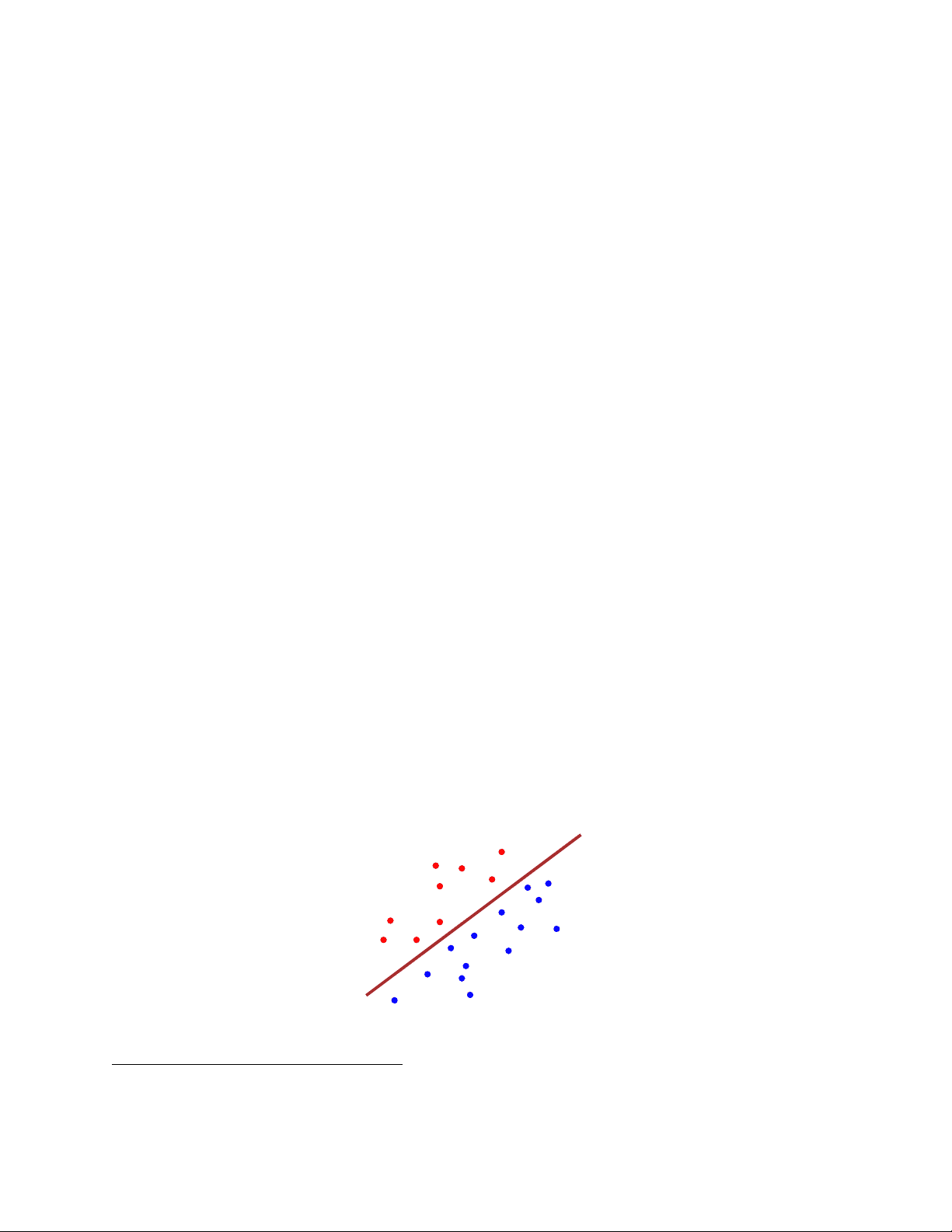
For example, consider a set of red and blue points,
`
Given the red and blue points, how to compute `?
¬ This work is licensed under the Creative Commons Attribution-Noncommercial 3.0 License. To view a copy of
this license, visit http://creativecommons.org/licenses/by-nc/3.0/ or send a letter to Creative Commons,
171 Second Street, Suite 300, San Francisco, California, 94105, USA.
This is a linear function:
f (
x ) =
a ·
x + b
Classification is sign( f (x)). If sign( f (x)) is negative, it outside the class, if it is positive it is
inside.
A set of examples is a set of pairs S = {(x 1 , y 1 ) ,... ,(xn, yn)} where xi ∈ IR
d and yi ∈ {-1,1}.
A linear classifier h is a pair (w, b) where w ∈ IR
d and b ∈ IR. The classification of x ∈ IR
d is
sign(x · w + b). For a labeled example (x, y), h classifies (x, y) correctly if sign(x · w + b) = y.
Assume that the underlying space has linear classifier (problematic assumption), and you are
given “enough” examples (i.e., n). How to compute this linear classifier?
Of course, use linear programming, we are looking for (w, b) s.t. for a sample
(xi, yi) we have sign(xi · w + b) = yi which is
xi · w + b ≥ 0
if yi = 1 and
→− xi ·
w + b ≤ 0
if yi = −1.
Thus, we get a set of linear constraints, one for each sample, and we need to solve this linear
program.
Problem: Linear programming is noise sensitive.
Namely, if we have points misclassified, we would not find a solution, because no solution satisfy-
ing all of the constraints, exist.
Algorithm Preceptron(S : a set of l examples)
w 0 ← 0,k ← 0
R = max(x,y)∈S
∥ x
repeat
for (x, y) ∈ S do
if sign(〈wk, x〉) , y then
wk+ 1 ← wk + y ∗
x
k ← k + 1
until no mistakes are made in the classification
return wk and k
Why does this work? Assume that we made a mistake on a sample (x, y) and y = 1. Then,
u = wk · x < 0, and
〈wk+ 1 , x〉 = 〈wk, x〉 + y 〈x, x〉 > u.
Namely, we are “walking” in the right direction.
Theorem 24.1.1 Let S be a training set, and let R = max(x,y)∈S
∥ x
∥.^ Suppose that there exists a
vector wopt such that
∥wopt
∥ =^1 and
y
wopt, x
≥ γ ∀(x, y) ∈ S.
We have: αk+ 1 ≤ αk − R
2 , and
α 0 =
R
2
γ
wopt
2
R
4
γ
2
∥wopt
2
=
R
4
γ
2
Finally, observe that
αi ≥ 0 for all i. Thus, what is the maximum number of classification errors the algorithm can make?
R
2
γ
2
It is important to observe that any linear program can be written as the problem of seperating
red points from blue points. As such, the Preceptron algorithm can be used to solve sovle linear
programs...
24.2 Learning A Circle
Given a set of red points, and blue points in the plane, we want to learn a circle that contains all
the red points, and does not contain the blue points.
σ
How to compute the circle σ?
It turns out we need a simple but very clever trick. For every point (x, y) ∈ P map it to the point
(
x, y, x
2
2
. Let z(P) =
x, y, x
2
2
∣ (x,^ y)^ ∈^ P
be the resulting point set.
Theorem 24.2.1 Two sets of points R and B are separable by a circle in two dimensions, if and
only if z(R) and z(B) are separable by a plane in three dimensions.
Proof: Let σ ≡ (x − a)
2
2 = r
2 be the circle containing all the points of R and having all
the points of B outside. Clearly, (x − a)
2
2 ≤ r
2 for all the points of R. Equivalently
− 2 ax − 2 by +
x
2
2
≤ r
2 − a
2 − b
2 .
Setting z = x
2
2 we get that
h ≡ − 2 ax − 2 by + z − r
2
2
2 ≤ 0.
Namely, p ∈ σ if and only if h(z(p)) ≤ 0. We just proved that if the point set is separable by a
circle, then the lifted point set z(R) and z(B) are separable by a plane.
As for the other direction, assume that z(R) and z(B) are separable in 3d and let
h ≡ ax + by + cz + d = 0
be the separating plane, such that all the point of z(R) evaluate to a negative number by h. Namely,
for (x, y, x
2
2 ) ∈ z(R) we have ax + by + c(x
2
2 ) + d ≤ 0
and similarly, for (x, y, x
2
2 ) ∈ B we have ax + by + c(x
2
2 ) + d ≥ 0.
Let U(h) =
(x, y)
∣ h
(x, y, x
2
2 )
. Clearly, if U(h) is a circle, then this implies that
R ⊂ U(h) and B ∩ U(h) = ∅, as required.
So, U(h) are all the points in the plane, such that
ax + by + c
x
2
2
≤ −d.
Equivalently
(
x
2
a
c
x
y
2
b
c
y
d
c
x +
a
2 c
2
y +
b
2 c
2
a
2
2
4 c
2
d
c
but this defines the interior of a circle in the plane, as claimed.
This example show that linear separability is a powerful technique that can be used to learn
complicated concepts that are considerably more complicated than just hyperplane separation. This
lifting technique showed above is calledlinearizion the kernel technique or linearizion.
24.3 A Little Bit On VC Dimension
As we mentioned, inherent to the learning algorithms, is the concept of how complex is the function
we are trying to learn. VC-dimension is one of the most natural ways of capturing this notion. (VC
= Vapnik, Chervonenkis,1971).
A matter of expersivity. What is harder to learn:
- A rectangle in the plane.
- A halfplane.
- A convex polygon with k sides.
Let X =
p 1 , p 2 ,... , pm
be a set of m points in the plane, and let R be the set of all halfplanes.
A half-plane r defines a binary vector
r(X) = (b 1 ,... , bm)
where bi = 1 if and only if pi is inside r.
Let
U(X, R) = {r(X) | r ∈ R}.