Download Computing MST, Generic Approach - Design and Analysis - Study Notes and more Study notes Digital Systems Design in PDF only on Docsity!
Lecture No. 35
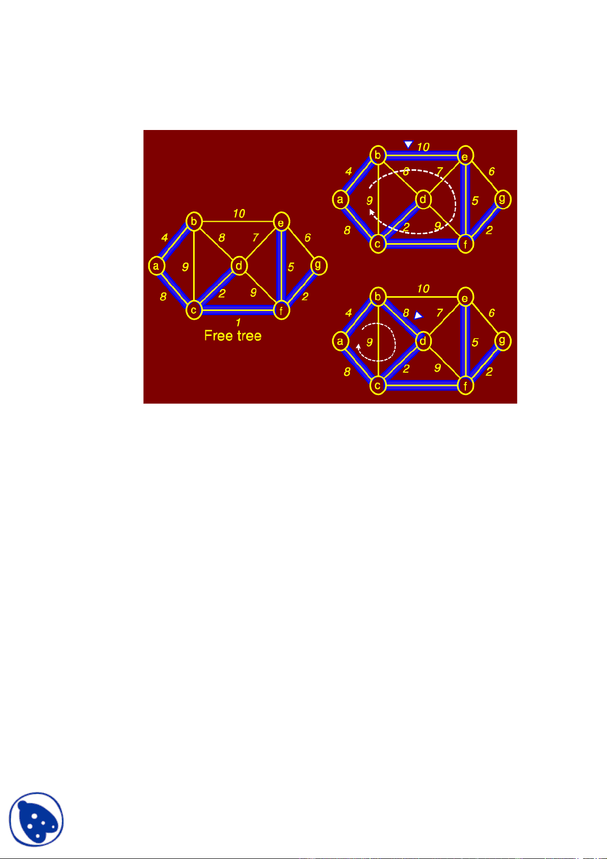
Figure 8.45: Free tree facts
8.5.1 Computing MST: Generic Approach
Let G= ( V, E) be an undirected, connected graph whose edges have numeric weights. The intuition behind greedy MST algorithm is simple: we maintain a subset of edges E of the graph. Call this subset A. Initially, A is empty. We will add edges one at a time until A equals the MST. A subset A ⊆ E is viable if A is a subset of edges of some MST. An edge (u, v) ∈ E- A is safe if A [ {(u, v)} is viable. In other words, the choice (u, v) is a safe choice to add so that A can still be extended to form a MST.
Note that if A is viable, it cannot contain a cycle. A generic greedy algorithm operates by repeatedly adding any safe edge to the current spanning tree.
When is an edge safe? Consider the theoretical issues behind determining whether an edge is safe or not. Let S be a subset of vertices S ⊆ V. A cut (S, V- S) is just a partition of vertices into two disjoint subsets. An edge (u, v) crosses the cut if one endpoint is in S and the other is in V-S.
Given a subset of edges A, a cut respects A if no edge in A crosses the cut. It is not hard to see why respecting cuts are important to this problem. If we have computed a partial MST and we wish to know which edges can be added that do not induce a cycle in the current MST, any edge that crosses a respecting cut is a possible candidate.
8.5.2 Greedy MST
An edge of E is a light edge crossing a cut if among all edges crossing the cut, it has the minimum weight. Intuition says that since all the edges that cross a respecting cut do not induce a cycle, then the lightest edge crossing a cut is a natural choice. The main theorem which drives both algorithms is the following:
MST Lemma: Let G = ( V, E) be a connected, undirected graph with real-valued weights on the edges. Let A be a viable subset of E(i.e., a subset of some MST). Let (S, V- S) be any cut that respects A and let (u, v) be a light edge crossing the cut. Then the edge (u, v) is safe for A. This is illustrated in Figure 8.46.
Figure 8.46: Subset A with a cut (wavy line) that respects A
MST Proof: It would simplify the proof if we assume that all edge weights are distinct. Let T be any MST for G. If T contains (u, v) then we are done. This is shown in Figure 8.47 where the lightest edge (u, v) with cost 4 has been chosen.
Figure 8.49: Cycle created due to T+ ( u , v)
Since u and v are on opposite sides of the cut, and any cycle must cross the cut an even number of times, there must be at least one other edge (x, y) in T that crosses the cut. The edge (x, y) is not in A because the cut respects A. By removing (x, y) we restore a spanning tree, call it T^0. This is shown in Figure 8.
We have w(T′) = w(T) - w(x,y) +w(u,v). Since (u,v) is the lightest edge crossing the cut we have
w(u, v) < w(x, y). Thus w(T′)< w(T) which contradicts the assumption that T was an MST.
8.5.3 Kruskal’s Algorithm
Kruskal’s algorithm works by adding edges in increasing ord er of weight (lightest edge first). If the next
edge does not induce a cycle among the current set of edges, then it is added to A. If it does, we skip it
and consider the next in order. As the algorithm runs, the edges in A induce a forest on the vertices. The
trees of this forest are eventually merged until a single tree forms containing all vertices.
The tricky part of the algorithm is how to detect whether the addition of an edge will create a cycle in A.
Suppose the edge being considered has vertices (u, v). We want a fast test that tells us whether u and v
are in the same tree of A. This can be done using the Union-Find data structure which supports the
following O (log n) operations:
Create-set(u): Create a set containing a single item u.
Find-set(u): Find the set that contains u
Union(u,v): merge the set containing u and set containing v into a common set.
In Kruskal’s algorithm, the vertices will be stored in sets. The vertices in each tree of A will be a set. The
edges in A can be stored as a simple list. Here is the algorithm: Figures 8.51 through 8.55 demonstrate
the algorithm applied to a graph.
K R U S K A L ( G = (V,E))
1 A ← {}
2 for (each u 2 V)
3 do create_set (u)
4 sort E in increasing order by weight w
5 for ( each (u, v) in sorted edge list)
6 do if (find(u) ≠ find(v))
7 then add (u, v) to A
8 union(u, v)
9 return A
Figure 8.54: Kruskal algorithm: (e, f)added
Figure 8.55: Kruskal algorithm: more unsafe edges and final MST
Analysis:
Since the graph is connected, we may assume that E≥ V- 1. Sorting edges ( line 4) takes Θ(E log E).
The for loop (line 5) performs O(E) find and O(V) union operations. Total time for union - find is
O(Eα(V)) where α(V) is the inverse Ackerman function. α(V) < 4 for V less the number of atoms in the
entire universe. Thus the time is dominated by sorting. Overall time for Kruskal is
Θ( E log E) = Θ( E log V) if the graph is sparse.
8.5.4 Prim’s Algorithm
Kruskal’s algorithm worked by ordering the edges, and inser ting them one by one into the spanning tree, taking care never to introduce a cycle. Intuitively Kruskal’s works by merging or splicing two trees together, until all the vertices are in the same tree.
In contrast, Prim’s algorithm builds the MST by adding leave s one at a time to the current tree. We start
with a root vertex r; it can be any vertex. At any time, the subset of edges A forms a single tree (in
Kruskal’s, it formed a forest). We look to add a single vertex as a leaf to the tree.
Figure 8.56: Prim’s algorithm: a cut of the graph
Consider the set of vertices S currently part of the tree and its complement ( V- S) as shown in Figure 8.56. We have cut of the graph. Which edge should be added next? The greedy strategy would be to add the lightest edge which in the figure is edge to ’u’. Once u is added, Some edges that crossed the cut are no longer crossing it and others that were not crossing the cut are as shown in Figure 8.
Figure 8.57: Prim’s algorithm: u selected
We need an efficient way to update the cut and determine the light edge quickly. To do this, we will make use of a priority queue. The question is what do we store in the priority queue? It may seem logical that edges that cross the cut should be stored since we choose light edges from these. Although possible, there is more elegant solution which leads to a simpler algorithm.
Figure 8.59: Prim’s algorithm: edges with weights 8 and 1 sel ected
Figure 8.60: Prim’s algorithm: the final MST
Analysis:
It takes O(log V) to extract a vertex from the priority queue. For each incident edge, we spend potentially O(log V) time decreasing the key of the neighboring vertex. Thus the total time is O(log V+ deg(u) log V). The other steps of update are constant time.
So the overall running time is
T(V, E) = u V ∈
∑ (log^ V+^ deg(u) log^ V)
= log V u V ∈
∑ (1^ +^ deg^ (u) )
= (logV)(V+2E) =Θ((V+E)logV)
Since G is connected, V is asymptotically no greater than E so this is Θ(E log V), same as
Kruskal’s algorithm.
8.6 Shortest Paths
A motorist wishes to find the shortest possible route between Peshawar and Karachi. Given a road map of Pakistan on which the distance between each pair of adjacent cities is marked Can the motorist determine the shortest route?
In the shortest -paths problem We are given a weighted, directed graph G= ( V, E) The weight
of path p=< v 0 , v 1 ,..., vk > is the sum of the constituent edges:
k
w(p ) =
i=
∑ w(vi-^1 , vi^ )
We define the shortest-path weight from u to v by
Problems such as shortest route between cities can be solved efficiently by modelling the road map as a graph. The nodes or vertices represent cities and edges represent roads. Edge weights can be interpreted as distances. Other metrics can also be used, e.g., time, cost, penalties and loss.
Similar scenarios occur in computer networks like the Internet where data packets have to be routed. The vertices are routers. Edges are communication links which may be be wire or wireless. Edge weights can be distance, link speed, link capacity link delays, and link utilization.
The breadth-first-search algorithm we discussed earlier is a shortest-path algorithm that works on un-weighted graphs. An un-weighted graph can be considered as a graph in which every edge has weight one unit.
There are a few variants of the shortest path problem. We will cover their definitions and then discuss algorithms for some.
Single-source shortest-path problem: Find shortest paths from a given (single) source vertex
s ∈ V to every other vertex v ∈ V in the graph G.
Single-destination shortest-paths problem: Find a shortest path to a given destination vertex t
from each vertex v. We can reduce the problem to a single-source problem by reversing the
direction of each edge in the graph.
Single-pair shortest-path problem: Find a shortest path from u to v for given vertices u and v.
If we solve the single-source problem with source vertex u, we solve this problem also. No
algorithms for this problem are known to run asymptotically faster than the best single- source algorithms in the worst case.