Download Handout 5: Multicollinearity - Lecture Notes | ECON 210 and more Study notes Introduction to Econometrics in PDF only on Docsity!
Economics 210
Econometrics
Handout # 5 Multicolinearity
The pro blem of multicolinearity exists when ther e exists a linear re lationship or an appro ximate linear re lationship among (between) two or more of the right hand side(RHS) variables( including the variable x 1 = 1 which generates the constant term) in a regression. There are two types of multicolinearity, perfect multicolinearity and near multicolinera rity.
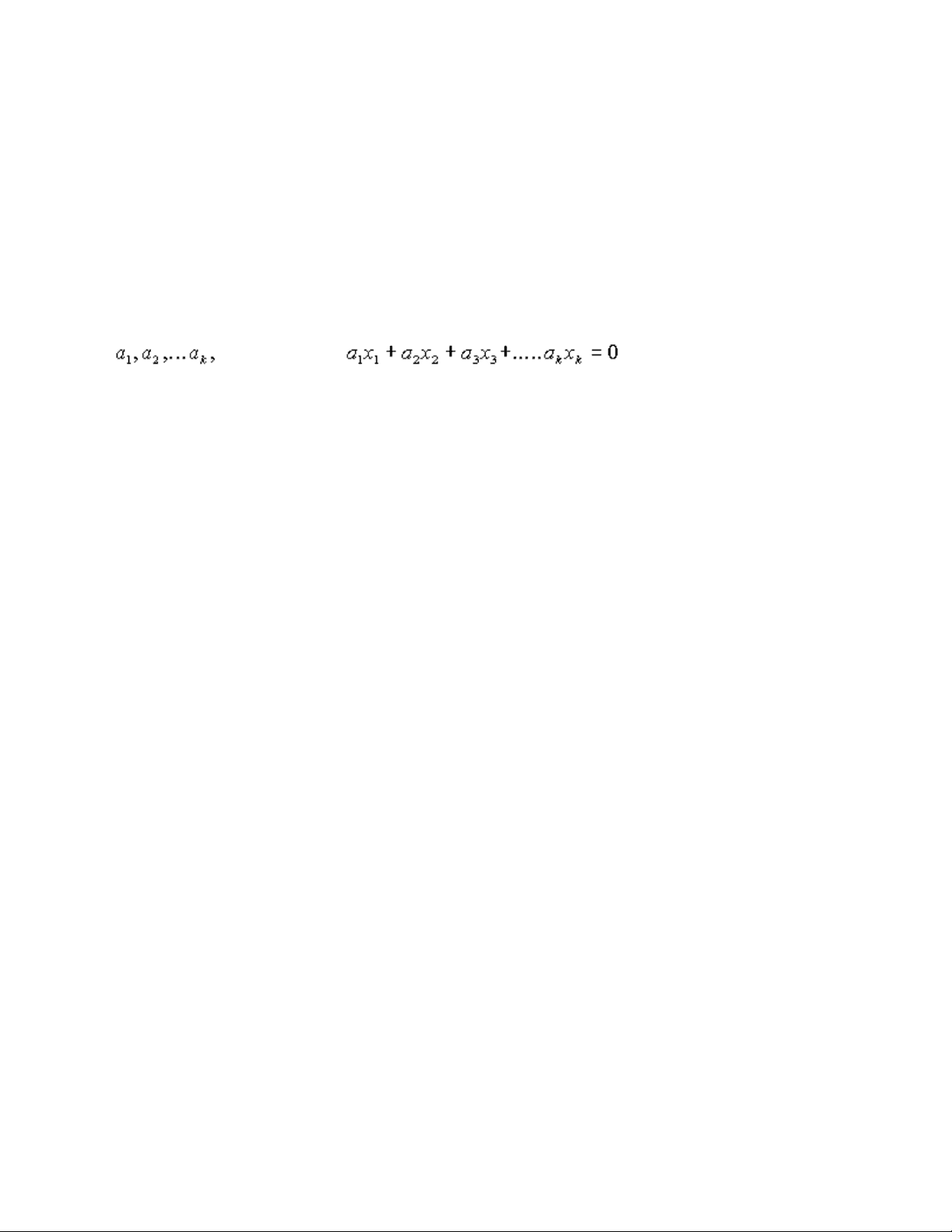
Perfect multicolinearity exists when there is some linear c ombinatio n of the RH S variables w hich is identically equal to zero. Form ally we say that perfect multicolinearity exists if there exists a set of coefficients,
not all 0, such tha t
Perfect multicolinearity is relatively rare and usually occurs because of the “dummy variable trap” or because the researcher has inadvertently included variables which are related by an id entity among the RHS variables.
Near multicolinearity is much mo re comm on. It occurs whenever so me or all of the right hand va riables are hig hly correlated.
Consequences of near multicolinearity for OLS.
- Estimator are BLUE but have high variances and covariances
- Low t ratio s, few coefficients sig nificant.
- Wide co nfidence intervals for individual coefficients.
- Although t ratios are statistically insign ificant, R-squar eds can b e high and F -tests of the joint hyp othesis that several coefficients are zero indicate that this hypothesis can be rejected.
- The estimated coefficients are very sensitive to small changes in the data or to changes in specification.
- High R-squareds and good fits are NOT a consequence of multicolinearity. There is sometimes some confusion a bout this po int.
Example I
reg x5-x
Source | SS df MS Number of obs = 100 ---------+------------------------------ F( 3, 96) = 46. Model | 5439.06109 3 1813.02036 Prob > F = 0. Residual | 3764.32783 96 39.2117482 R-squared = 0. ---------+------------------------------ Adj R-squared = 0. Total | 9203.38892 99 92.9635244 Root MSE = 6.
y | Coef. Std. Err. t P>|t| [95% Conf. Interval] ---------+-------------------------------------------------------------------- x5 | 3.74287 2.189337 1.710 0.091 -.6029292 8. x6 | -.4550604 4.465227 -0.102 0.919 -9.318465 8. x7 | .9309749 2.282723 0.408 0.684 -3.600193 5. _cons | 201.0018 .6339865 317.044 0.000 199.7433 202.
This a classic example o f multicolinearity. N one of the co efficients of the exp lanatary variab les are significantly different than ze ro at a 5% level of significanc e. But the R -squared is .5 9 and F tes t indicates that the h ypothesis that the coefficients of all of the explanatory variables are equal to zero can be rejected. So we can conclude that some variable or variables in the set x5, x6, x7 has explanatory power but we cannot tell which variable or what the individual coefficients are.
vif
Variable | VIF 1/VIF ---------+---------------------- x5 | 49.98 0. x6 | 49.22 0. x7 | 8.57 0. ---------+---------------------- Mean VIF | 35.
Suppose that we run the re gression dropping the first nine and the last ten ob servations:
reg y x5-x7 in 10/
y | Coef. Std. Err. t P>|t| [95% Conf. Interval] ---------+-------------------------------------------------------------------- x5 | 1.508106 2.517559 0.599 0.551 -3.504994 6. x6 | 3.771561 5.151895 0.732 0.466 -6.487174 14. x7 | 3.584481 2.623777 1.366 0.176 -1.640127 8. _cons | 200.7715 .7325884 274.058 0.000 199.3127 202.
Notice the change in the coefficients when we change the data on which the estimations are based. This is additional evidence of multicolinea rity.
Now suppose we drop o ne of the explanatory variables from the regression.
reg y x5 x
R-squared = 0. Adj R-squared = 0.
y | Coef. Std. Err. t P>|t| [95% Conf. Interval] ---------+-------------------------------------------------------------------- x5 | 4.580231 .7567498 6.053 0.000 3.078292 6. x6 | -2.161079 1.555281 -1.390 0.168 -5.247881. _cons | 200.9988 .631214 318.432 0.000 199.746 202.
reg y x6 x
R-squared = 0. Adj R-squared = 0.
y | Coef. Std. Err. t P>|t| [95% Conf. Interval] ---------+-------------------------------------------------------------------- x6 | 7.098166 .6530677 10.869 0.000 5.802008 8. x7 | 4.590801 .8002566 5.737 0.000 3.002513 6. _cons | 200.9791 .6400991 313.981 0.000 199.7087 202.
Note that in each case the coefficients of the remaining variables change dramatically. Note also that the R-squared and the Adjusted R-squared do not change very much. (In fact, when we drop the variable x7 the Adjusted R- squared increases.
Example II
reg y x2-x
Source | SS df MS Number of obs = 100 ---------+------------------------------ F( 6, 93) = 74. Model | 7622.82135 6 1270.47023 Prob > F = 0. Residual | 1580.56756 93 16.9953502 R-squared = 0. ---------+------------------------------ Adj R-squared = 0. Total | 9203.38892 99 92.9635244 Root MSE = 4.
y | Coef. Std. Err. t P>|t| [95% Conf. Interval] ---------+-------------------------------------------------------------------- x2 | 2.298464 .4266107 5.388 0.000 1.451299 3. x3 | -5.676951 4.493383 -1.263 0.210 -14.59992 3. x4 | 10.43627 4.577264 2.280 0.025 1.346729 19. x5 | 2.795344 1.449848 1.928 0.057 -.083766 5. x6 | .1417058 2.954301 0.048 0.962 -5.724951 6. x7 | 1.833148 1.51105 1.213 0.228 -1.167497 4. _cons | 200.5923 .4212379 476.197 0.000 199.7558 201.
vif
Variable | VIF 1/VIF ---------+---------------------- x4 | 109.15 0. x3 | 108.64 0. x5 | 50.57 0. x6 | 49.71 0. x7 | 8.66 0. x2 | 1.10 0. ---------+---------------------- Mean VIF | 54.
The VIF results indicate that at least four of the explanatory variables and maybe a fifth are involved in multicolinearity.
reg y x2 x4-x
y | Coef. Std. Err. t P>|t| [95% Conf. Interval] ---------+-------------------------------------------------------------------- x2 | 2.30275 .4279479 5.381 0.000 1.45305 3. x4 | 4.680917 .4478829 10.451 0.000 3.791635 5. x5 | 2.94777 1.449394 2.034 0.045 .0699647 5. x6 | -.0885397 2.958011 -0.030 0.976 -5.96174 5. x7 | 1.680369 1.510972 1.112 0.269 -1.319702 4. _cons | 200.5432 .4207682 476.612 0.000 199.7077 201.
Notice the change in the coefficient of x4 when the variable x3 is dropped from the regression. The other coefficients do not change much indicating that there is a linear relationship between x3 and x4.
reg x3 x2 x4-x
R-squared = 0.
x3 | Coef. Std. Err. t P>|t| [95% Conf. Interval] ---------+-------------------------------------------------------------------- x2 | -.0007551 .0097922 -0.077 0.939 -.0201977. x4 | 1.01381 .0102484 98.924 0.000 .9934617 1. x5 | -.02685 .0331647 -0.810 0.420 -.0926993. x6 | .0405579 .0676845 0.599 0.550 -.0938313. x7 | .0269122 .0345737 0.778 0.438 -.0417347. _cons | .0086516 .0096279 0.899 0.371 -.0104649.
. reg x4 x2 x3 x5-x
Source | SS df MS Number of obs = 100 ---------+------------------------------ F( 5, 94) = 2033. Model | 87.7327757 5 17.5465551 Prob > F = 0. Residual | .811181966 94 .008629595 R-squared = 0. ---------+------------------------------ Adj R-squared = 0. Total | 88.5439577 99 .894383411 Root MSE =.
x4 | Coef. Std. Err. t P>|t| [95% Conf. Interval] ---------+-------------------------------------------------------------------- x2 | -.0003983 .009613 -0.041 0.967 -.0194851. x3 | .9769935 .0098762 98.924 0.000 .9573841. x5 | .0281849 .0325407 0.866 0.389 -.0364254. x6 | -.0420456 .0664296 -0.633 0.528 -.1739431. x7 | -.0282021 .0339249 -0.831 0.408 -.0955607. _cons | -.0075836 .0094597 -0.802 0.425 -.026366.
. reg x5 x2 x3 x4 x6 x
R-squared = 0.
x5 | Coef. Std. Err. t P>|t| [95% Conf. Interval] ---------+-------------------------------------------------------------------- x2 | -.005963 .0303428 -0.197 0.845 -.0662094. x3 | -.2578967 .3185505 -0.810 0.420 -.8903862. x4 | .2809203 .3243348 0.866 0.389 -.363054. x6 | 2.013683 .0321486 62.637 0.000 1.949851 2. x7 | .9781113 .0371177 26.352 0.000 .9044132 1. _cons | -.0053849 .0299617 -0.180 0.858 -.0648746.
Note: The following approximate relationships exist among the variables
x4 = x x5 = 2x6 + x We can rewrite the equation:
We can estimate this last equation by regressing y on x2, x3,x6 and x7.