Download Handout VIII: Time Series and Distributed Lag Models | ECON 310 and more Study notes Econometrics and Mathematical Economics in PDF only on Docsity!
Economics 310
Handout # VIII Time Series and Distributed Lag Models
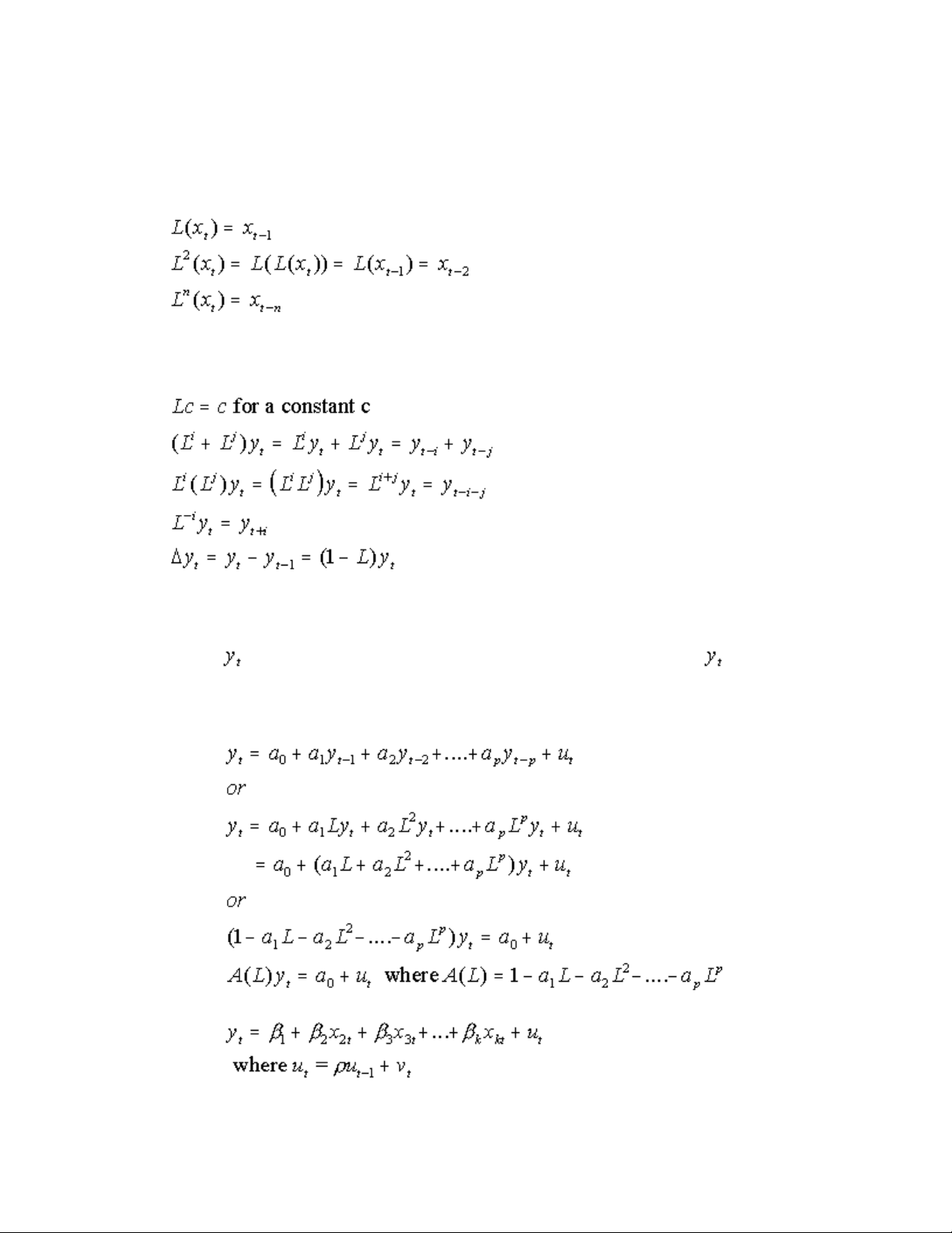
A. Lag Operators : A lag operator generates the lagged value of a variable
Properties of Lag Operators
Autoregressive Processes
Def: If is a function of its own lagged values and an error term, then is called an autoregressive process. The order of an autoregressive process is the maximum number of lags. In general an autoregressive process of order p, AR(p), can be written as
We have been using autoregressive processes for some time. For example
Lag polynomials can be manipulated algebraically. For example
Distributed Lag Models and Autoregressive Models
Model 1. Distributed Lags
Typical problems with this model are i) too many regressors and ii) multicolinearity
Estimation: Polynomial Distributed Lags Geometric Distributed Lags
Model 2. Geometric Distributed Lags
Suppose that in the distributed lag model the effect of variable diminishes as the lag gets
larger. Specifically let’s assume that
Substituting into the distributed lag model we get
This transformation is know as a Koyck transformation.
Estimation
Each of models 2, 3, and 4 lead to the equation In models 2 and
3 the error term is of the form while in model 4. If we knew the
distribution of in the original model then we would know the distribution of. For example
if we knew that the were serially uncorrelated the would be serially uncorrelated in the
model 4 and negatively serially correlated in the models 2 and 3. If there was serial correlation
in the errors the transformations in models 2 and 3 would have changed the structure of the
serial correlation. However, usually we have no prior knowledge of the distribution of the.
The question of whether the errors are serially correlated is of crucial importance in selecting an appropriate estimation procedure.
Case I. No serial correlation. Then and will be uncorrelated and OLS will produce
consistent estimators. (There will be small sample bias.)
Case II. If is serially correlated then there is contemporaneous correlation between and
and OLS will produce biased and inconsistent estimates.
A complicating factor is that the Durbin-Watson statistic is biased toward the value 2 (indicating an absence of serial correlation) if a lagged y value is present as an explanatory variable. In this case a alternative test for serial correlation should be used.
Some form of instrumental variables estimation is usually used if serial correlation is present.