Download Quantum Mechanics of Electrons: Wave-Particle Duality and Energy Levels and more Study notes Chemistry in PDF only on Docsity!
light
beam
slit
screen
diffracted
pattern
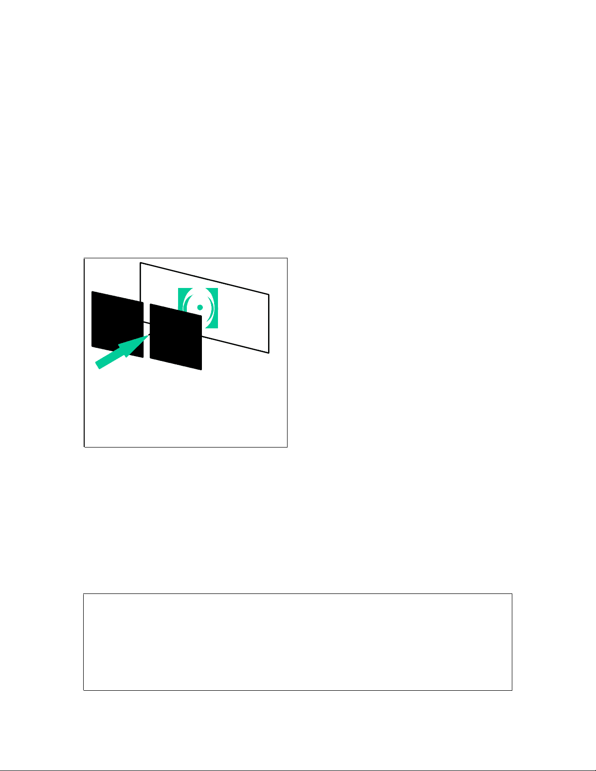
Fig. 1. When a single color light beam passes through a slit, it creates a diffraction pattern (a series of bright and dark spots or rings) on the white screen behind the slit. Lecture Series 3 Chem 20A James Heath Recall that we concluded our discussion of the discoveries by Planck, Einstein, and Bohr by stating that the single theme that ran through those discoveries was that, at very small length scales, various physical phenomena were no longer continuous, but rather discrete , or quantized. Light, as well as matter, also comes in discrete units – the photon. Electrons, which are discrete particles of matter orbit a nucleus in discrete orbits that are characterized by discrete angular momenta. Now there is one more piece of information that we need before we can proceed to a more applicable description of quantum mechanics. When we described electromagnetic radiation (light), we described it as both waves, and as discrete packets of energy (photons). This wave/particle duality is not unique to light. In fact, it is very general. Some time after the three paradoxes were confronted by Planck, Bohr, and Einstein, other scientists began doing experiments on electrons, and finding some very puzzling results. It was well known (from Newton’s time), that if light was sent through a very small slit, it would diffract, as shown in Fig. 1. This is how diffraction gratings work, and also why a rainbow is a rainbow.. Some scientists began doing this same experiment with electrons. They would make a beam of electrons, send it through a slit, and look at a phosphoroscent screen placed behind the slit. What they found was rather surprising. They observed diffraction patterns, just as if they had done the experiment with a beam of light! This implied that electrons – which had previously been considered to be particles – also had wave-like characteristics. Based on these results and the other work that was being done by Planck, Louis de Broglie wrote a very brief doctoral thesis in which he postulated that all matter was characterized by a wavelength, and that wavelength could be calculated from the following equation: = h/mv = Planck’s constant divided by the momentum of the particle. This equation was in agreement with the observed diffraction measurements Example: Say that we had a beam of electrons, travelling with a kinetic energy of 10, eV’s (1 eV = 1.6x10⁻¹⁹J). What is the wavelength associated with those electrons? (By the way, eV’s are a very convenient unit to use here. If we accelerate an electron through an electric field of x volts, the that electron has a kinetic energy of x eV.) So, if kinetic energy = 1x 10^4 eV = ½ mv^2 , then the momentum = mv. We know that m = me = 9.1 x 10⁻³¹^ kg, so we can solve for v, and hence momentum.
Figure 2. A guitar string and its resonant frequencies. Notice that all frequencies are integral multiples of the fundamental frequency, shown at the bottom of the drawing. 104 eV ( 1.6 x 10⁻¹⁹J/eV) = ½(9.1 x10⁻³¹^ kg)(v^2 ): v = 5 x 10^7 m/s = (6.63x10⁻³⁴^ J s)/[( 1x10^4 eV)(1.6x10⁻¹⁹^ J/eV)(5 x 10^7 m/s)]-1^ = 1.2 x 10⁻¹¹^ m = 0.1 Angstroms. If we had used protons instead of electrons, would = 3 x 10-13^ m – a quantity that is essentially not measureable! As objects get more and more massive, their momentum increases, and the wavelengths associated with them get smaller and smaller
- quickly becoming too small to measure. We know that mass and light each have wave-like and particle-like characteristics, and that electrons in atoms are quantized – they have discrete energies, or, equivalently, they have discrete values of the angular momenta. We have so far presented only the facts. Now we try to ask why. Our first question: Why does an electron become quantized? Quantum mechanics is not a particularly intuitive subject, and so analogies to real world phenomena are a little dangerous. Nevertheless, here is one that works a little bit. Imagine that we have a guitar string, tied down at either end, as if it were on a guitar. If we pluck the string, then we hear a note, and this note is the resonance frequency of the string. This is, of course, the basis for all stringed instruments. One selects an appropriate string, puts an appropriate tension on that string, and stretches it across some length. These things we do to the string will give it a desired resonant frequency – say an ‘A’ note. Now it turns out that when you pluck the string, you not only hear the ‘A’ note, but if you listen very closely, you will hear an ‘A’ note at the next octave up, and even the 2d^ octave up as well, and so on and so forth. These are harmonics, and their frequencies are integral multiples of the first primary note, or the fundamental frequency. This is shown graphically in Fig. 2. In the language of physics, let’s restate the various phenomena that control the resonance frequency of the string: First, we have the mass of the string – larger mass translates to lower resonance frequencies. Second, we have the tension on the string. When we stretch a string, we are actually using it as a spring – i.e. if we let loose of both ends, it will retract back to its initial length. When we pull or compress a string (or a spring) this is the same as increasing its potential energy. When we compress or expand a spring, we store energy into the spring in the form of potential energy. Thus, the amount of potential energy stored in the string is important: More potential energy (tighter string) corresponds to higher resonance frequencies. Third, we have the length of the string that is resonating. Shorter lengths lead to higher frequency resonances. This is why frets are on a guitar.
length Energy E 3 E 1 E 2 Fig. 5. Now we redraw our previous figure that described the resonances of a string to represent the resonances of a confined electron. The dots on the length-axis are the dots of Fig. 3. Note the energy spacings increase as n^2. Let’s work this out a little bit. If we have a box of length L, then, according to Figs 2 and 4, the fundamental frequency has a wavelength of 2L. (Notice how only ½ of the fundamental wavelength fits into the box.) 2L = h/mv, so mv = h/2L and so v = h/(2Lm) = h/(m). Energy = kinetic energy + potential energy. However, if we keep our particle within the boundaries of the box, then the potential energy = 0, so the total Energy = the kinetic energy = ½ mv^2. So if E = ½ mv^2 , the energy of the fundamental is given by Ef = ½ m (h^2 /4L^2 m^2 ) = ½ h^2 /(4L^2 m) = h^2 /(8mL^2 ). Let’s go to the 1st^ overtone. = L = h/mv, so v = h/mL. E (^) 1st ov. = ½ mv^2 = ½ m h^2 /m^2 L^2 = h^2 /(2mL^2 ) = 4h^2 /(8mL^2 ) And, for the 2d^ overtone, = 2/3 L = h/mv, so v = 3/2 h/mL and E2d ov. = ½ mv^2 = ½ m 9h^2 /(4m^2 L^2 ) = 9h^2 /8mL^2 So we have a series of states with En = n^2 (h^2 /8mL^2 ), where the fundamental frequency has n = 1, the 1st^ overtone has n = 2, the 2d^ overtone has n = 3, etc. Here, n is the quantum number that denotes a quantum state of the system. En is the energy of the nth^ state. There is a function that describes the 3 waves shown in Fig. 4 (and all the other ones that aren’t shown), and that function is called the wave function of the system. Each of the separate waves is a quantum state of the system, and each state is characterized by a quantum number. The wave function is often denoted by the symbol , or ‘psi’. Notice that the quantum number determines the shape of the wave function. If we had really set up a differential equation and solved this problem as your book does, we would have also found that En = h^2 n^2 /(8mL^2 ). It turns out that the reason our approach works is because this is an unrealistic, but very simple system: the potential energy contribution to the total energy of the system was negligible. Thus, other than using the potential energy to define how big our box was, we neglected it when we calculated the energy of the system. Usually we can’t do this. So let’s go back to the factors that affected the resonance frequency of the guitar string (mass of string, potential energy, length of string), and ask how those factors affect the properties of our quantum mechanical waves. First, however, we need to adopt a slightly different representation for our waves. Since we know that shorter wavelengths correspond to higher kinetic energies, we can represent the fundamental frequency and it harmonics as shown in Fig. 5. First, we had the mass of the string – larger mass translated to lower resonance frequencies. Here, we have fixed by L, the length of the box to which the electron is
confined. However, we also still have the relationship: = h/mv. Thus, if is fixed, and we increase mass, then the velocity of the particle decreases. Recall, once again, our favorite equation for energy: E = ½ mv^2. If the product mv stays the same (since the wavelength doesn’t change), yet the mass is increased, then velocity must proportionately decrease. The energy only varies linearly with mass, but it varies as the square of the velocity. Thus, a small increase in mass plus a small change decrease in velocity translates into decrease in kinetic energy. Increasing mass reduces the energy of the wave. Second, we had the tension on the string. More potential energy (tighter string) corresponded to higher resonance frequencies. Our situation is similar. In the particle-in-a-box, the potential energy is what keeps the particle restricted to a small part of the axis. If we remove the potential energy barriers (remove the dots in Fig. 3), then the electron is no longer confined to a particular part of the axis, and it can have all ranges of wavelengths associated with it, including very long ones. Third, we had the length of the string that was resonating. Shorter lengths led to higher frequency resonances. In fact, if we reduce the width of the box , we shorten the wavelength – just like in the case of a guitar. But we also increase the energy of the electron. If is reduced, then momentum (mv) is increased, and hence kinetic energy of the electron is increased.
One Last Background Point – The Heisenberg Uncertainty Principle
There is one more thing we need to cover before we get to a real quantum
mechanical system (the atom), and it is called the Heisenberg Uncertainty
Principle. This principle is fundamental to quantum mechanics – it is not strictly
provable, but, like the rest of quantum mechanics, it has withstood the test of time
admirably.
In any measurement that we can imagine doing, we will always have a little
bit of uncertainty in our answer – that uncertainty is governed by our
instrumentation, or by the nature of the thing we are trying to measure. Let’s say
that we are trying to measure the position of an electron. The only way we can do
this is to scatter something off of the electron – like a photon. When we do this,
we may get a very accurate measurement of where the electron was at the time of
the scattering event, but we have also changed the system. Imagine, for example,
that the electron is travelling along with some velocity v in some direction, giving
it a momentum p = mass x velocity. If we scatter a photon off of the electron in
order to measure its position, then we change its momentum. We don’t really
know how we change it, but we change it. So now, if we try to measure its
momentum, which we can do, it is not the same momentum that it had when we
measured its position. – confusing, huh? What Heisenberg showed is that if we
try to measure both the position and the momentum of an electron, then the
precision of our position measurement, times the precision of our momentum
measurement, must be greater than h/4. We can write this as px h/4,
where the is read as ‘the uncertainty in.’ Let’s do an example:
(it is a volume surrounding the positive nucleus), we know that there will be 3 quantum numbers describing the electron – one quantum number corresponding to each degree of freedom. Thus, we already see one of the problems with Bohr’s atom – it only has one quantum number. So if we need one quantum number per degree of freedom, then what are those degrees of freedom? If we had a particle in a 3-dimensional box, we might just call them x, y, and z, and get quantum numbers nx, ny, and nz. However, that is not what we have. Instead, we have a particle (the electron) held within some region of space by a centro-symmetric Coulombic potential (the positive nucleus). One obvious degree of freedom that we have is a measurement of how far out from the nucleus is the electron – i.e. what is its radial distance. The quantum number corresponding to this is the radial quantum number. If we decide on this as one of our quantum numbers, then what are the other two? Look at Figure 6. Here we show that we can describe the position of the electron by r, its distance from the origin, and by the angles theta () and phi (). These are related to the xyz coordinate system because is the angle of r within the xy plane, and is the angle that (the vector) r makes with the with respect to the z-axis. Let’s not worry about this too much, other than that we need one degree of freedom to describe the distance of the electron from the origin, and two degrees of freedom that describe angles. Thus, we have one radial quantum number, and two angular quantum numbers. The radial quantum number will dictate how the wavefunction spreads out from the nucleus, and the two angular quantum numbers will determine the shape of the wavefunction.
Quantum numbers of electronic orbitals
The wave function of an electron is usually denoted by . For the case of the electron orbiting around the nucleus, as is shown in Fig. 6, is a function of r, , and . The energy levels of the electron are described by the three quantum numbers n (the principal, or radial quantum number), l , or the angular momentum quantum number, and m , which is called the magnetic quantum number. We’ll return to these quantum numbers in a minute. We write as nlm (r,,), and we find that we can separate into a radial component R nl (r) and lm (,), so that we can write: nlm (r,,) = R nl (r) lm (,) We also find that there are certain relationships between the quantum numbers, and we’ll describe those in a minute. I just list this information so that you see that there are three quantum numbers, and three degrees of freedom. What do those quantum numbers mean? – We don’t know yet. If we had set up and solved an equation that described Fig. 6, which is a hydrogen-like atom, we would have been able to derive all of the stuff that is being presented here. This is a very difficult thing to do, and is usually not attempted until the last year of an undergraduate chemistry program, or the first year of a graduate chemistry program. Nevertheless, what we would have found would have been just a more complicated version of the ‘quantum guitar string’ problem we solved earlier. Just like the guitar string, the energy levels would have been described by an energy En, where n is the principal quantum number: En = -Z^2 e^4 me(8o^2 n^2 h^2 )-1,
Let’s define the constants in this energy expression. Z is the nuclear charge. For H atom, it is simply 1, for Li2+, it is 3, and for He+^ it is 2. Why is this? H has one proton, so one positive charge. Li2+^ has 3 protons, so a positive nuclear charge of +3, and He+^ has 2 protons. We don’t worry about neutrons since they are charge neutral. Also all of these atoms are hydrogen-like – meaning that there is just one electron orbiting about a positive charge. Even though the magnitude of the positive charge differs, the physical solutions work out to be the same -- they are just scaled for the different charges. You should understand this concept. Going back to the equation for En – we have e^4 , which is the fundamental unit of charge to the 4th^ power, we have me, which is the mass of the electron. In the divisor, we have o^2 , the constant that corresponds to the permittivity of a vacuum (squared). We have h^2 , which is Planck’s constant squared, and we have n^2 , which is the primary or radial quantum number squared. Thus, just like our quantum guitar string, the energy of a given quantum state is related to only one quantum number n. However, unlike the solution to the quantum guitar string, the energy depends inversely on n, scaling as n-2. This means that if we plot the energy levels of this system as a function of n, they will look something like what is shown in Fig. 7. The energy levels that describe our hydrogenlike system do not depend upon the other two quantum numbers l and m. However, a given En describes the energy of one or more quantum states of the system. Those quantum states are, more or less, electronic orbitals, and they have a shape. It is the shape of those wavefunctions, which is related to the orbital angular momentum, that is determined by the quantum numbers l and m. We could have solved for the shapes and angular momentum of these various states, and we would have found that n, l, and m have certain relationships with one another. n = 1, 2, 3, 4, …. l = 0, 1, 2, .. (n-1) m = - l , - l +1, - l +2, … 0, l -2, l -1, l So, for example, if n = 3, what are the possible combinations of other quantum numbers that we could have? n = 3, l = 2, m = -2, -1, 0, 1, 2 n = 3, l = 1, m = -1, 0, 1 n = 3, l = 0, m = 0 What are the allowed quantum numbers if we have n = 1? n = 4? You should be able to figure this out yourself. When we want to describe a particular orbital, there are some nomenclature rules. First, we consider the principal quantum number n. Then we consider the angular momentum quantum number l. If l = 0, it is an s-orbital. If l = 1, it is a p-orbital, and if l = 2, it is a d-orbital. Other less commonly encountered orbitals include f-orbitals ( l =3) and g- orbitals ( l =4). Returning to the case of n = 3, we have l =0,1,or 2. These combinations yield 3s, 3p, and 3d orbitals. So how about m? It turns out the number of values for m describe the number of 3s, 3p, or 3d orbitals. For example, for a 3s orbital, m can only be
length
Energy
E 1 node E 2 Figure 8. The ‘quantum guitar string,’ but only the first two energy states are drawn. The point where the wave function passes through the dashed lines is called a node. 0 1s r 0 2s r node 0 3s r nodes Fig. 9. The radial wavefunctions of 1s, 2s, and 3s orbitals. Note how the number of nodes increases from 1 to 2 to 3. As the wavefunction passes through a node, its sign changes, just like a sin function passing through 0o. 2pz z x y 2py 2px Fig. 10. 2p orbitals. First, we consider the s-orbitals. For all s- orbitals, both l and m are 0. What this means is that the orbital does not really have much angular shape – it is simply a sphere, radiating outward from the positive nuclear core. But how about n? This quantum number affects the radial part of the wavefunction (the function Rnl(r) at the top of this section). As we move from n=0 to n=1 to n=2, etc. the principle quantum number is changing, so the radial part of the wavefunction must change. In fact, this change is very similar to what we observed for our quantum guitar string. Recall that as we increased n, we moved from the fundamental frequency to higher harmonics. Let’s look at that graph one more time, and discuss terms. In Fig. 8 we have redrawn the lowest two states of the quantum guitar string, with a couple of additions. We have drawn dashed lines through the strings, indicating the nodes in the function. When a wave function passes through the dashed line, it changes sign. We call the point at which it crosses a node. Consider a sin function. sin(0o) = 0. sin(1o) > 0, and sin(-1o) < 0. Thus, when sin(angle) passes through 0o, it passes through a node. Now return back to one of the earlier figures of these waves – one that shows the first three states. Notice how the first state has 0 nodes, the second state has 1 node, and the 3rd^ state has 2 nodes. It turns out that the nth^ state would have (n-1) nodes. The radial wavefunction that describes the electronic orbits is very similar. For n=1, it has 0 nodes. For n=2, it has 1 node. For n = 3, it has 2 nodes, and so on and so forth. However, unlike the quantum guitar string, the radial function it not symmetrically bound by infinite potential barriers, so it looks different. The n=1, 2, 3 radial functions for l = 0 are shown in Fig. 9. If one is given a radial wavefunction, then just count the number of nodes, add 1, and you have the principle quantum number. Something that is implied by this statement is that a wavefunction with more nodes is a higher energy wavefunction. Since these wavefunctions are spherically symmetric (the situation for l and m both = 0), they look like concentric rings of opposite sign, radiating out from the positive nuclear core. In your text you will find graphs of the 1s, 2s, and 3s orbitals, shown to highlight these nodes. So how about if l = 1 or something other than 0? This implies that we have shape to our wavefunction – i.e. its structure is a little more interesting than just a spherical orbital. Notice that the radial part of the wavefunction (the equation given early in this section) is given as R nl (r), so it depends on both n and l. For n = 2, we know that R nl (r)
Energy n= n= n= 0 1 2 1s 2s 2p 3s 3p (^) **3d
__**
__
1s
__ 1s will have 1 node. If l = 1, then it turns out that the node is at the nucleus, not some distance out from the nucleus such as is shown for the 2s orbital in Figure 9. For n=2, l =1, we have p-orbitals, and we have the possible values for m of –1, 0, or 1. It turns out that the fact that l = 1 means that the p-orbitals are going to have the shape of two stacked eggs, aligned along some axis. These orbitals are shown in Figure 10. The three values of m define which axis the p-orbital is aligned along, and we will arbitrarily say that for m = -1, the p-orbital is aligned along z. If m = 0, it is aligned along x, and if m = 1, it is aligned along y. Since the wavefunction of a 2p orbital changes sign as it passes through the nucleus, one of the two eggs will have one sign (i.e. is positive), while the other egg has another sign (i.e. is negative). For example, in the 2pz orbital at the top of Fig. 10, if the top egg is positively signed, then the lower egg is negative. Just like the radial functions drawn in Fig. 9, if the wavefunction passes through a node, then it always changes sign. For n=3 and l =2, we again have d-orbitals – the 3d orbitals. We aren’t going to worry about these too much in this class. Nevertheless, there are 5 3d-orbitals, and they each have two nodes. Pictures of them are in your text.
Filling the Orbitals
Let’s list the various orbitals for n = 1, 2, and 3 in a slightly different way, but once again with energy as the y-axis (Fig. 11). This is similar to Fig. 7, except that we have replaced the individual labels of the m quantum number with just a series of empty spaces (underline marks). Each empty space stands for an unoccupied orbital, and so Fig. 11 represents a system with no electrons. So how do we fill these orbitals up with electrons? There are several rules. Let’s state two now:
_1. fill lowest energy orbitals first
- each orbital can hold two electrons_ So let’s start filling. For the first two electrons, its easy: We fill in the following way: and then: We call these two configurations 1s^1 and 1s^2 , respectively. The superscript at the right of these notations stands for the number of electrons in the orbital. Note that when we fill these orbitals, we are denoting the individual electrons with a little arrow, either pointing up or down. We’ll get back to that in a minute. So far, we have built the H atom and the He atom. Now we move down to the next atom, which is Li. We are faced with a choice. Apparently, all of the 2s and 2p orbitals are degenerate , meaning that they are at the same energy level. Thus, where do we put the electrons? It turns out that all of the orbitals of same principle quantum number are degenerate only for hydrogen and
2p
__ __ __
2p
__ __ __
2p
__ __ __
2p
__ __ __ Ne
O
N
B
Fig. 13: Filling the p- orbitals using rule #4. Energy
n=
n=
n=
1s 3s
___
2s
__
__
n=
4s
__
3p
__ __ __
3d
__ __ __ __ __
4p
__ __ __
2p
__ __ __
Figure 14. The energy ordering of the atomic orbitals for the first 4 rows of the periodic table. Note that the 3d orbitals are at lower energy than the 4p orbitals. down. If it held any more, then we would have a violation of the Pauli exclusion principle. It turns out that spin is a real physical quantity, but all we need to know is that two electrons can exist in the same orbital only if they have opposite spin. So, how does the spin quantum number guide us when we put together a carbon atom? This gives us rule #4.
- When filling orbitals that have the same n and l quantum numbers (but different m), first put one electron into each orbital, keeping all electron spins the same. Once all the orbitals are filled with one electron, each with the same spin, then finish filling the orbitals by pairing those electrons. In Fig. 13, we show how this is done for much of the 2p series. Assume in this figure that the atoms already have a 1s^2 2s^2 configuration that is not shown. We are just worrying about the 2p configuration. In Fig. 14, we show, for the n = 1, 2, and 3, and some of 4, how the orbitals line up in energy. You should be able to use this diagram, plus the rules stated here, to predict the ground state electronic configuration of pretty much any atom in the first 4 rows of the periodic table. This is the end of what will be covered by the first midterm.
END LECTURE SERIES 3