Download Particle-Wave Duality in Quantum Mechanics and more Lecture notes Quantum Mechanics in PDF only on Docsity!
Matthew Schwartz
Lecture 20:
Quantum mechanics
1 Motivation: particle-wave duality
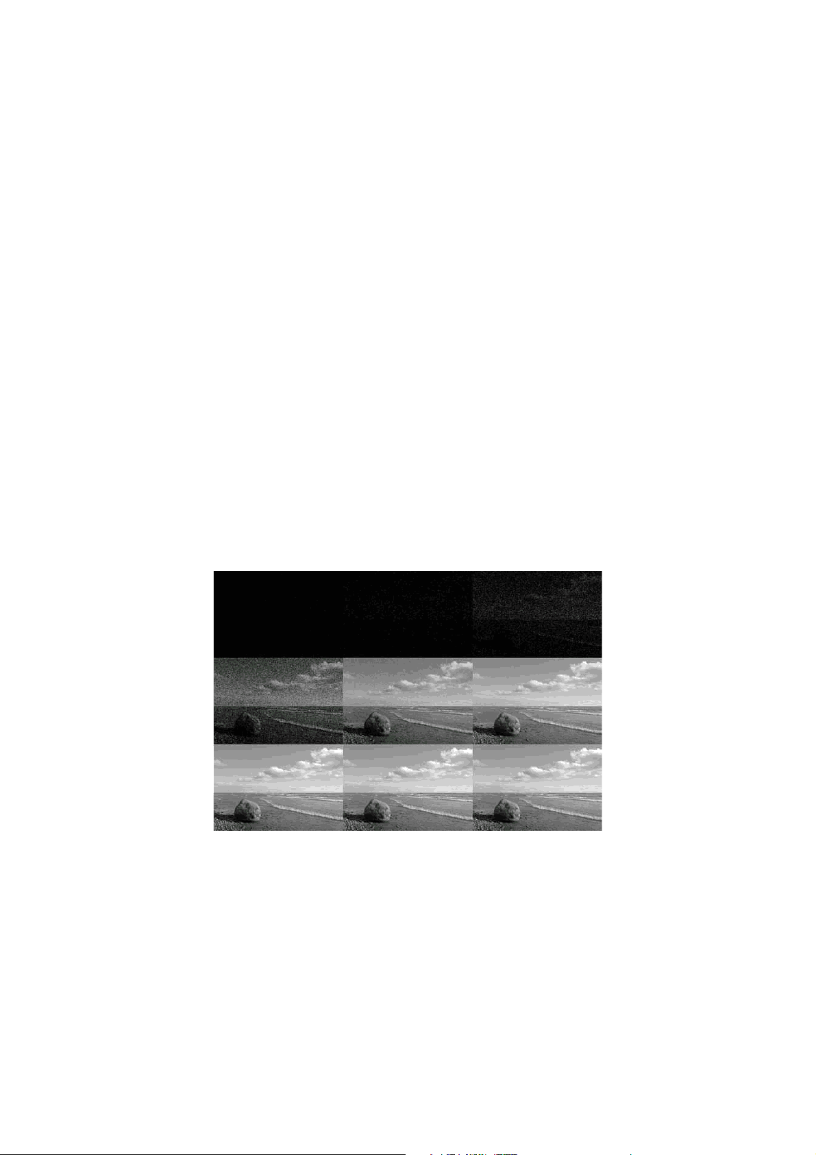
This has been a course about waves. We have seen how light acts like a wave in many contexts – it refracts, diffracts, interferes, disperses, etc. Light also has a paricle-like nature. Newton was the first to propose this, based mostly on observations about ray-tracing in geometrical optics. For example, that shadows had sharp edges were evidence to Newton that light was made of particles. This was in the 17th century. However, all of Newton’s observations are perfectly con- sistent with light as a wave. Geometric optics is simply the regime when the wavelength of light is much smaller than the relevant scales of the apparatus. Over the next 200 years, as the wave theory was developed by physicists such Fresnel, Huygens and Maxwell, the particle-like nature of light was basically accepted as wrong. However, light is made of particles. An easy way to see this is with a digital camera. Digital cameras are wonderfully more sensitive than film cameras. As we discussed in Lecture 17 on color, as you pump up the “ISO” on a digital camera, you are pumping up the gain on the CCD. That is, you change the mapping from intensity to the number 0-255 recorded at each pixel. At very high ISO such as 6400, you can be sensitive to single photon depositions on your sensor. Suppose we take a light source and add more and more filters in front of it to reduce the inten- sity and take pictures of it. The result looks like this
Figure 1. Going from bottom right to top left, nine photos of the same scene are taken with more and more light filtered out. The graininess of the images is mostly due to shot noise: there are a finite number of photons hitting the camera.
The type of graininess that results from the finite number of photos in light is called shot noise (There are other sources of graininess, such as sensor imperfections, but shot noise dominates at low light). If you thought light was just a wave, when you lower the intensity, you would expect the photo to just get dimmer and dimmer at lower light. That there are dots in discrete places is evidence that the intensity is produced by particles hitting the sensor. If you take the same pic- ture again at low light, the dots show up in different places. So there is an element of random- ness to the locations of the photons.
We have seen that classical electromagnetic waves carry power. This is obvious from the fact that they can induce currents. By setting electrons into motion, the energy of the wave goes into kinetic energy in the electron motion. Electromagnetic waves also carry momentum. Again, this is easy to see classically: if a wave hits an electron at rest, the oscillating electric field alone would only get it moving up and down, like a cork on water when a wave passes. However, once the electron is moving, the magnetic field in the wave pushes it forward, through the F = eB × v
force law. The electron is pushed in the direction of the wavevector k~^ , thus the momentum in a
plane wave is proportional to ~k^.
So if light is made of particles, those particles must be carrying momentum ~p , and this ~p
must be proportional to the wavevector ~k^. We write ~p = ℏ ~k^. By dimensional analysis, this con- stant ℏ must have units of J · s. We write ℏ = 2 hπ and the value observed is
h = 6.26 × 10¹⁹ J · s (1)
known as Planck’s constant. Since ω = c
∣~k
∣ (^) for electromagnetic radiation, and since light is
massless, mc^2 = E^2 − c^2 ~p^2
= 0 we find that E = c|~p | = ℏc
∣~k
∣ (^) = ℏω = hν, so energy is propor-
tional to frequency for light.
Of course, there were no digital cameras when quantum mechanics was invented. The key experimental evidence for photons came from careful studies of shining light on metals. By 1900, it was known that shining light could induce a current in a conductor. Interestingly though, the induced current depended not just on the intensity of the light, but also on its frequency. For example, in potassium, it was found that low intensity blue light would induce a current but high-intensity red light would not. The current is induced in a metal because light hits elec- trons, which are then freed to move around. In some situations, an even more dramatic effect occurs: the electrons get ejected from the metal. This is called the photoelectric effect. In 1902, Philipp Lenard found that the energy of the ejected electrons did not depend on the inten- sity of the light, but only on its frequency. A high frequency light source would free lots of elec- trons, but they would all have the same energy, independent of the intensity of the light. A low- frequency light source would never free electrons, even at very high intensity.
These observations are explained by quantum mechanics. The basic observation is that elec- trons have a binding energy Ebind in a metal. One needs a minimal amount of energy to free them. This binding energy is itself not a quantum effect. For example, we are bound the the earth; it takes a minimum amount of energy Em in = 12 m vesc^2 with vesc = 11.2 km s the escape velocity to set us free. Quantum mechanics plays a role through the identification of frequency
with energy: because photons have energy E = hν it takes a minimum frequency νm in = Eb i n d h to free the electron. After that, the electron will have kinetic energy Ekin = Ebind − hν. So one can make a precise prediction for how the velocity of the emitted electron depends on energy 1 2 m v
(^2) = Ebind − hν. This relation between v and ν was postulated by Albert Einstein in 1905
and observed by Robert Millikan in 1914. Both were later awarded Nobel prizes (as was Lenard).
Two other important historical hints that classical theory was wrong were the classical insta- bility of the atom and the blackbody paradox. The classical instability is the problem that if atoms are electrons orbiting nuclei, like planets orbiting the sun, then the electrons must be radiating power since they are accelerating. If you work out the numbers (as you did on the problem set), you will see that the power emitted is enormous. So this classical atomic model is untenable and must be wrong.
The blackbody paradox is that classically, one expects a hot gas to spread its energy evenly over all available normal modes. This evenness can actually be proved from statistical mechanics; the general result is known as the equipartition theorem. Now say you have light in a finite volume, such as the sun. It will have normal mode excitations determined by boundary conditions. Treating the volume like a box whose sides have length L, these will have wavevectors ~k^ = (^2) Lπ ~n , where n~ is a vector of integers, e.g. ~n = (4, 5 , 6). Since ω = c
∣~k
∣ (^) in three
dimensions there are many more modes with higher frequency than lower frequency. If these all
2 Section 1
Since intensity is just photon counts, we expect this pattern will slowly build up if we shine the light at low intensity. That is just what happens, as can be seen in Figure 4 :
Figure 4. Double slit interference pattern at low intensity. The pattern accumulates slowly, going from panel 3, to panel 2, to panel 1. Eventually, the granularity in the intensity pattern would wash out and it would match what we get with high intensity light over a shorter time.
This figure is equivalent to zooming in on the central region in the bottom right panel of Figure 3 and lowering the intensity. It is also true that if you cover up one of the slits, you find the single-slit interference pattern accumulating over time, as in the top right panel of Figure 3.
Now if you start to think about it is a little, this result is very weird. The intensity pattern accumulates even if the intensity is very low, say one photon per minute. But if only one photon is going through at a time, what is it interfering with? Certainly not other photons. The answer is, it is interfering with itself! The photon must be going through both slits at once. Otherwise the interference pattern couldn’t possibly be affected by closing off one slit.
To make this even clearer, you can do the same experiment with electrons. Exactly the same thing happens: the electrons produce an interference pattern if both slits are open, but no inter-
ference pattern if one slit is closed. For the photon case, the pattern was I(y) = 4I 0 cos^2
π (^) λLdy
with λ the photon’s wavelength.
What is the “wavelength” of an electron? Well, for light momentum was ~p = ℏ~k^ and
∣~k
∣ (^) = 2 π λ. Thus, the wavelength of light can be extracted from its momentum as λ = 2 ∣∣π k~^ ∣∣ = (^) |~hp |. It is natural
to expect that this equivalence will also work for electrons. This definition is called the de Broglie wavelength
λ ≡ h |~p |
This de Broglie wavelength correctly determines the scale for the interference pattern in the electron double slit experiment.
Continuing this logic, the electron’s wavevector is ~k^ = (^1) ℏ ~p and the electron’s angular fre-
quency is ω = (^1) ℏ E, with E the electron’s energy. From special relatively, we know that the elec-
tron’s energy is E = m^2 c^4 + p^2 c^2
. Thus electrons satisfy the dispersion relation
ℏω = m^2 c^4 + ℏ^2 c^2 ~k^2
This has a low-frequency cutoff (like in a plasma): the frequency of the electron satisfies ω > m c^2 ℏ. Another useful quantity with units of length is the Compton wavelength of the electron
λc = h mc
= 2.42 × 10 −^12 m (4)
4 Section 2
Unlike the de Broglie wavelength, the Compton wavelength does not depend on momentum. The Compton wavelength is just a translation of the electron mass into length units and repre- sents, roughly, the length scale where quantum mechanics becomes relevant. Calling it a wave- length is somewhat inappropriate. It should more appropriatelly be called the Compton length scale. The de Broglie wavelength really is the wavelength of the wave that a particle with momentum p has. So all the interference effects and so on depend on the de Broglie wavelength. The Compton wavelength does not directly characterize the scale for interference; it is merely a length scale that comes up in a lot of quantum mechanics calculations, as in Eq. ( 17 ) below, so it is handy to give it a name.
3 The Schrödinger equation
So light is made of particles that act like waves. Electrons are also particles which act like waves. We will now focus mostly on electrons. The reason is that to we want to focus on just one particle at a time, and with photons it’s hard to do that. Due to E = mc^2 and that m = 0 for a photon, it is very easy to produce a lot of light. Indeed, there is no good regime where we can study single photons without having to consider multiple photons. Quantum field theory is quantum mechanics in regimes where energies are greater than the threshold for producing pairs of new particles with E = mc^2. For photons, this threshold energy is zero. For electrons, it is twice the rest mass, 2 me ≈ 1.5 × 10 −^13 J ≈ 1 MeV. This is an enormous amount of energy, not generated in the laboratory until the 1930’s.
What is the wave equation for the electron? To deduce it, we can work backwards from the dispersion relation. For electrons, plane waves ψ(x, t) = exp(iωt − ikx) with the dispersion rela- tion in Eq. ( 3 ) would satisfy the wave equation
[ ℏ^2
∂^2
∂t 2
+ ℏ^2 ∇~^
2
]
ψ(x, t) = 0 (5)
with ψ(x, t) the amplitude of the electron, more commonly called its wavefunction. Eq. ( 5 ) is called the Klein-Gordon equation.
The solutions to the Klein-Gordon equation are plane waves, or linear combinations of plane waves. However, we are not usually interested in what happens to an electron pummeling through free space. Instead, we like to study systems with lots of positively and negatively charged particles, like atoms, molecules and solids. For example, around a proton, the electron is influenced by the background V (r) = q
2 4 πε 0 r Coulomb potential. So, let’s adapt the Klein-Gordon equation a little so it’s more practical. First of all, in most situations, the kinetic energy of the electron is much less than its rest mass (if this weren’t true, we’d need quantum field theory). So it makes sense to Taylor expand the mass-energy relation:
E = m^2 c^4 + p^2 c^2
= mc^2 + p
2 2 m +^ ···. To include the stuff around the electron, we can include the fact that the energy of the electron can also be modified in the presence of some potential V (x), like around a proton or a nucleus. So E = mc^2 + p
2 2 m +^ V^ (x) +^ ···. In fact, since only energy dif- ferences are ever measurable, we might as well absorb the rest mass into this potential. So we now have E = ~p
2 2 m +^ V^ (x). Note that since^ ~p^ =^ m v~^ the^
p~ 2 2 m =^
1 2 m v~
(^2) is just the ordinary non-rela-
tivisitic kinetic energy. In terms of the frequency and wavevector, ω = E ℏ and^ k
~ (^) = ~p ℏ , this becomes ℏω = ℏ^2 k
~ 2 2 m +^ V^ (x)^ and the wave equation becomes [ iℏ
∂t
ℏ^2
2 m
∇~^2 − V (x)
]
ψ(x, t) = 0 (6)
The Schrödinger equation 5
Figure 5. Visible hydrogen emission spectrum.
It is perhaps useful to note that conservation of energy translates to conservation of fre- quency. This isn’t that different from what we have seen classically: a driven oscillator moves at the frequency of the driver. As waves pass across different media, the frequency is fixed, but the wavelength changes.
5 Wavepackets
The wavefunction ψ(x, t) is the amplitude. So |ψ(x, t)|^2 gives the intensity. As we saw in Sec- tion 2 , however, the intensity for single photons or single electrons does not show up as a very faint smooth pattern, but rather as discrete dots. The reason behind this is one of the hardest parts of quantum mechanics to get your head around. The way it works is that |ψ(x, t)|^2 gives the probability of finding an electron at a position x and t. This probability interpretation is often taken as a postulate of quantum mechanics, although really it follows from careful consid- eration of entanglement with the surroundings. Let’s just take the probability interpretation as given. For V = 0, the Schrödinger equation is simply [ iℏ
∂t
ℏ^2
2 m
∇~^2
]
ψ(x, t) = 0 (11)
This is called the free Schrödinger equation. It has plane wave solutions
ψ(~ , tx ) = eiωt−ik~^ ·~x^ (12)
where ω and k~^ satisfy the dispersion relation ω = ℏk
~ 2 2 m. Where are the electrons in the plane wave? The probability of finding one at a point ~x at time t is |ψ(x~ , t)|^2 = 1. Thus they are everywhere! Clearly plane waves are not useful for describing electrons in any regime where they act particle-like. There are lots of other solutions to the free Schrödinger equation besides the plane wave ones. For example, we can construct wave-packets. As in Lecture 11, we can write at t = 0
ψ(~x ) = e − (^12)
( (^) ~x −x~ (^0) σx
) 2 ei k~^0 ·x~^ (13)
this is a packet centered at ~x = ~x 0 with width σx and a carrier wavelength ~k 0. The Fourier trans- form is
ψ˜(k) = σx (2π)3/^
e
− (^12)
( (^) k −k 0 σk
) 2 e−ix^0 (k−k^0 )^ (14)
with σk = (^) σ^1 x
. This is a wavepacket centered on k~ 0. But ~p = ℏ~k^. So the momentum distribution
is Gaussian too.
Wavepackets 7
In fact, just as |ψ(~x )|^2 gives the probability that we find the electron at the position ~x at
time t, it is also true that
ψ˜
~k
gives the probability that we find the electron with momentum ~p = ℏ~k^. Thus the most likely value for momentum is ~p 0 = ℏ k~ 0 and the width of the
momentum distribution is σp = ℏσk = (^) σℏ x
. In particular, we find
σxσp = ℏ (15)
This is a special case of the Heisenberg uncertainty principle
(∆x)(∆p) > ℏ (16)
(sometimes you see this relation with ℏ 2 on the left; the factor of 2 has to do with precisely how
∆x and ∆p are defined). This says that for any wavefunction, the uncertainty on position ∆x times the uncertainty of momentum ∆p must be larger than or equal to ℏ. Gaussian wavepackets saturate this inequality. Note that ℏ = 1.04 × 10 −^34 J ·s is very small. So we can actually know the position and momentum of the electron quite well at the same time – to less than 10−^17 each in SI units. Quantum mechanics only shows this weird uncertainty if you are at very short distances. Next, note that the carrier wavenumber k 0 translates to the most likely momentum value. In position space, we see from Eq. ( 13 ) that the phase of the wavefunction gives the momentum. Thus a wavefunction at a given time has both position information (in the amplitude) and momentum information (in the phase).
What happens to these electrons with time? Since the dispersion relation ω = ℏk
~ 2 2 m is not linear, there is dispersion. That is, wavepackets broaden over time. As we saw in Lecture 11, the second derivative of the frequency with respect to wavenumber determines the broadening rate.
In this case, Γ = ω′′(k 0 ) = (^) mℏ is independent of k 0. In terms of the Compton wavelength in Eq.
( 4 ), Γ = 2 λπcc. Then the width grows (see Eq. (36) of Lecture 11) as
σ(t) = σx 1 +
λcct 2 πσx^2
λc 2 πσx
ct (17)
where the last form holds at late times. So no matter how localized the electron is at t = 0, eventually, we will lose track of it. For example, suppose we start out knowing the electron
down to σx = λc = 10 −^12 m. Then at late time σ(t) = (^21) π c t. Thus the electron wavepacket is broadening at the speed of light. Moreover, the smaller σx we start out with, the faster the packet broadens. We can take σx large to slow the broadening, but for large σx, we don’t know where the electron is to begin with. Electrons are very hard to pin down indeed!
8 Section 5