Download River of Life and Determinats and more Study Guides, Projects, Research Construction Procedures in PDF only on Docsity!
4 Determinants
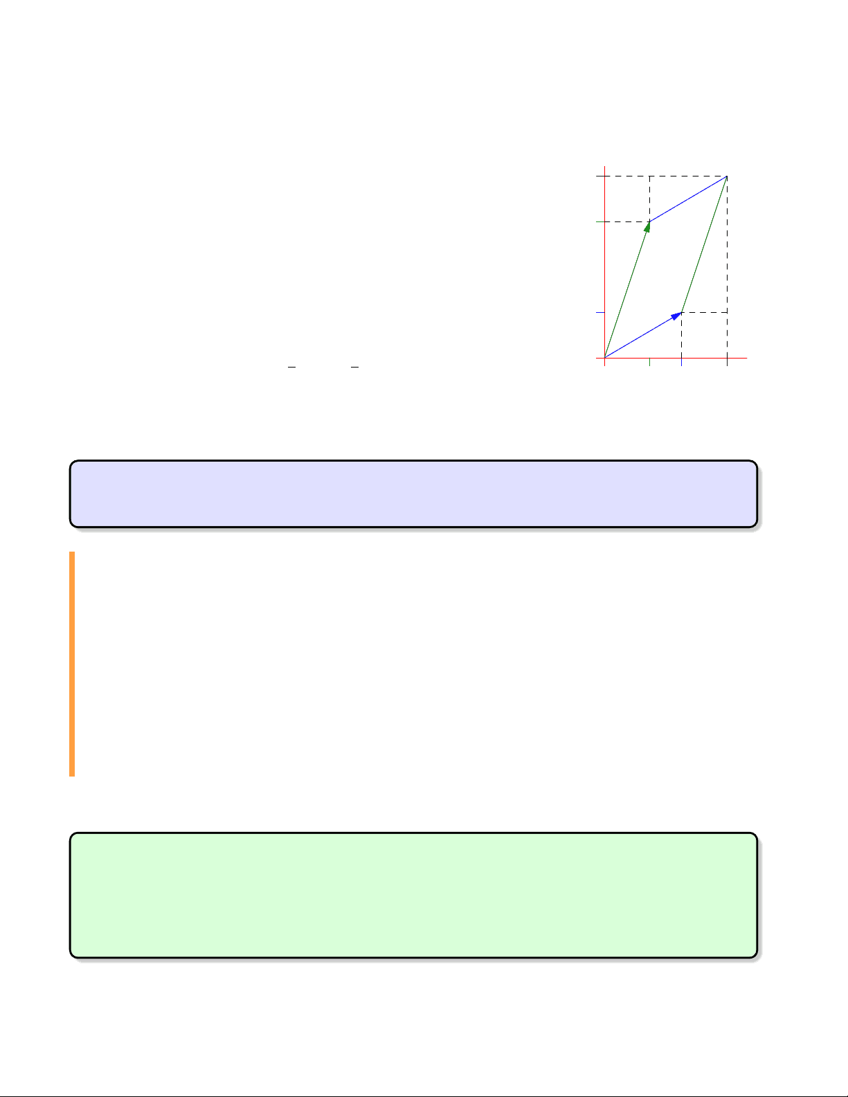
To a square matrix A, it turns out that we can attach a single number, its determinant, which encapsu- lates the extent to which the linear map LA enlarges or contracts space. For instance, consider a 2 × 2 matrix A =
� (^) a b c d
. Its columns are the result of multiplying the standard basis vectors i , j by A:
A i =
a c
A j =
b d
For simplicity, suppose a, b, c, d > 0 and that the columns are ori- ented as in the picture. The unit square spanned by i , j is transformed by A to a parallelogram, whose area is
(a + b)(c + d) − 2 bc − 2 ·
bd − 2 ·
ac = ad − bc
A i
A j
a
d
c
b a + b
c + d
This one number neatly summarizes how left-multiplication by A changes the area of a shape.
4.1 Determinants of Order 2
Definition 4.1. The determinant det A = |A| of a 2 × 2 matrix A =
� (^) a b c d
is the scalar
det A = ad − bc
Example 4.2. If A =
4 3
and B =
1 − 2
, then
det A = 1 · 3 − 2 · 4 = −5, det B = 5 · (− 2 ) − 0 · 1 = − 10
Note that det : M 2 ( F ) → F is a non-linear function; for instance
det(A + B) =
= 6 − 10 = − 4 ̸= det A + det B
However, determinant does play nicely with matrix multiplication:
det AB =
= − 42 + 92 = 50 = det A det B
In the following results, we summarize the key properties of order 2 determinants: with the exception of the explicit inverse formula, these will eventually be seen to hold in higher dimensions.
Theorem 4.3 (Basic properties of order-two determinants). 1. det AT^ = det A
- det A = 0 if and only if the columns (rows) of A are parallel (linearly dependent).
- Determinant is a bilinear function of the columns (rows) of A.
- det AB = det A det B
These are easily verified directly: write A =
� (^) a b c d
, B = ( p qr s ), etc. The third property benefits from a little expansion: writing a matrix in terms of its columns, determinant can be thought of as a function
det : F^2 × F^2 → F : ( a 1 a 2 ) 7 → det( a 1 a 2 )
and property 3 claims that
det( λ u + v , w ) = λ det( u , w ) + det( v , w ) and det( u , λ v + w ) = λ det( u , v ) + det( u , w )
and similarly with regard to the rows of a matrix (a pair of row vectors).
Example 4.4. The fact that the first rows are identical means we can combine
− 24 = − 5 − 19 = det
= det
Properties 2 and 3 partly overlap with the effect of row/column operations on determinant.
Corollary 4.5 (Row/column operations).
Type I: Swapping rows (or columns) changes the sign of det A Type II: Multiplying a row (or column) by λ multiplies det A by λ Type III: Adding a multiple of one row (or column) to another leaves det A unchanged
Proof. Simply combine the product formula with the list of all elementary matrices
det EA = det AE = det E det A
Type Matrices Determinant I
1 0
det E = − 1 II
� (^) λ 0 0 1
0 λ
det E = λ III
� (^1) λ 0 1
λ 1
det E = 1
Alternatively you can compute all possibilities directly.
Corollary 4.6 (Inverses). A is invertible (non-singular) if and only if det A ̸= 0. In such a case, det A−^1 = (^) det^1 A and
A =
a b c d
=⇒ A−^1 =
det A
d −b −c a
Proof. (⇒) If A is invertible, the product formula tells us that
1 = det I 2 = det(AA−^1 ) = det A det A−^1 =⇒ det A ̸= 0 and det A−^1 =
det A (⇐) Observe that � a b c d
d −b −c a
ad − bc 0 0 ad − bc
= (det A)I 2
If det A ̸= 0, we divide by det A to see that A has an inverse given by the desired expression.
Exercises 4.1 1. Compute the determinants of the following matrices and, if possible, their inverses:
(a)
7 − 3
∈ M 2 ( R ) (b)
� (^) i 1 +i 1 i
∈ M 2 ( C ) (c)
1 4
∈ M 2 ( Z 5 ) (d)
3 4
∈ M 2 ( Z 5 )
(Recall that Z 5 = {0, 1, 2, 3, 4} is the field of remainders modulo 5)
- Explicitly prove all parts of Theorem 4.3.
- Find the area of the triangles (a triangle is half a parallelogram... ):
(a) With vertices (0, 0), (2, 4) and (1, − 2 ). (b) With vertices (2, 1), (3, − 2 ) and (−5, 4).
- (a) Show that the matrix R = √a (^21) +c 2 ( (^) −ac a^ c ) acts by counter-clockwise rotation. (Hint: the columns of R are related by
1 0
( (^) −ac ) = ( ca )) (b) Complete the proof of Theorem 4.8.
- Let F be a field and ∆ : F^2 × F^2 → F be a bilinear function: ∀ u , v , w ∈ F^2 , λ ∈ F ,
∆( λ u + v , w ) = λ ∆( u , w ) + ∆( v , w ) and ∆( u , λ v + w ) = λ ∆( u , v ) + ∆( u , w )
(a) We say that ∆ is alternating if ∆( u , u ) = 0 for all u ∈ F^2. i. Prove that ∆ alternating =⇒ ∆( v , u ) = −∆( u , v ) for all u , v. ii. Prove the converse to part (a) (provided 2 ̸= 0 in F !). (b) Prove that if ∆ is an alternating bilinear function satisfying ∆( i , j ) = 1, then ∆ = det.
- (A link to multivariable calculus) Let D, E ⊆ R^2 and T : D → E be a change of co-ordinates
T(u, v) =
x(u, v), y(u, v)
Assume T is bijective and that the partial derivatives of x, y with respect to u, v exist and are continuous. Note that T does not have to be linear! Let P = (u 0 , v 0 ) ∈ D, and consider small positive quantities ∆u, ∆v to define points
Q = (u 0 + ∆u, v 0 ), R = (u 0 , v 0 + ∆v)
The area of the parallelogram spanned by
PQ = i ∆u and
PR = j ∆v is therefore ∆u∆v.
Prove that the parallelogram spanned by
T(P)T(Q) and
T(P)T(R) has
Area ≈ det
xu(P) xv(P) yu(P) yv(P)
∆u∆v
where xu = ∂ ∂ ux , etc., denote partial derivatives. This determinant is the Jacobian J(T) = ∂ ∂ ((xu,,yv)). The above is essentially the justification for the change of variables formula for double integrals: ZZ
E
f (x, y) dxdy =
ZZ
D
f
x(u, v), y(u, v)
� (^) ∂ (x, y) ∂ (u, v)
dudv
4.2 Higher-Order Determinants
We now extend the definition of determinant to any size of square matrix. The goal is to establish all the basic properties seen for order 2 determinants. This will take a little time...
Definition 4.9. Let A ∈ Mn( F ). For each i, j we defined the ijth^ minor of A to be the matrix A˜ij obtained by deleting the ith^ row and jth^ column of A. The determinant of A to be the sum
det A =
n
j= 1
(− 1 )^1 +j^ a 1 j det ˜A 1 j = a 11 det ˜A 11 − a 12 det ˜A 12 + · · · + (− 1 )^1 +n^ a 1 n det ˜A 1 n
This is known as the cofactor expansion of det A along the first row of A.
The difficulty should be immediately obvious: the definition is inductive! For instance the determi- nant of A ∈ M 4 ( F ) is defined in terms of the four 3 × 3 determinants, each of which is computed using three 2 × 2 determinants: in total we need twelve order 2 determinants!
Example 4.10. Let A =
0 1 2 − 1 −2 3 2 6 1 2 1 1
, then
det A = 1
Next we compute the remaining 3 × 3 determinants using the cofactor expansion:
det A =
1 1 −^2
2 1 + (−^1 )^
2 1 −^
1 1 + (−^1 )^
2 1 −^
1 1 +^2
Each of the remaining 2 × 2 determinants can now be evaluated:
det A = − 4 − 2 (− 9 ) − (− 1 ) − 2 (− 8 ) − 2 (− 7 ) − 3 (− 4 ) + 6 (− 7 ) = 15
While the above calculation was assisted by the fact that we only needed to compute three 3 × 3 determinants, it is still very slow-going. As the order n gets larger, things becomes ugly very quickly. In order to facilitate more rapid calculations it is useful to develop some of the properties we saw in the previous section. We begin by computing the determinant of the n × n identity matrix In: The
Examples 4.13. 1. Look for rows with many zeros when computing the determinant! Compare, for instance, the cofactor expansions of the following along the first and second rows:
First row: det
0 0 2 7 2 1
Second row: det
0 0 2 7 2 1
- Here we take advantage of linearity and the fact that the first two rows are nearly identical before expanding along the second row of the resulting 3 × 3 determinant:
det
1 2 3 0 1 2 0 − 1 1 0 2 5
1 2 3 4 1 2 3 4 1 2 0 − 1 1 0 2 5
1 2 3 4 0 0 0 4 1 2 0 − 1 1 0 2 5
1 2 3 1 2 0 1 0 2
Elementary matrices and the determinant
We now consider the effect of elementary row operations on the determinant.
Corollary 4.14. Let A be an n × n matrix and let E an elementary matrix. For each type:
Type I: det EA = − det A, and det E = − 1 ;
Type II: If E multiplies a row by λ , then det EA = λ det A, and det E = λ ;
Type III: det EA = det A and det E = 1.
Warning! Multiplying every row by λ yields det( λ A) = λ n^ det A
It is worth taking stock for a moment:
- For order two determinants (Corollary 4.5) these results followed from the multiplicative prop- erty det AB = det A det B.
- For higher order, we need to prove directly (using Theorem 4.12). Indeed the Corollary estab- lishes the limited multiplicative property det EA = det E det A whenever E is elementary. We will use this fact in the next section to prove the full multiplication formula.
Proof. 1. See Exercise 4.2.
- Suppose E = E i( λ )multiplies row i by λ. Since det is linear in each row, we immediately see that det EA = λ det A.
- Suppose E( ik λ )adds λ times row k to row i. Since determinant is linear in row i, we see that
det EA = det A + λ det B
where B is the matrix obtained from A by replacing row i with row k. Since B has two identical rows, we conclude that det EA = det A.
Letting A = In in each case gives the advertised values for det E.
Examples 4.15. 1. In case the argument for part 3 of the theorem is unclear, here is an example: if
E = E 21 (^5 ) =
5 1
and A =
3 − 1
, then
B =
and det EA = det
= det
- We can use all the above results to assist us in computing determinants. For instance,
det
=^0 +^3
- 0 (cofactor expansion 2nd^ row)
(type III row operations simplify third rows)
(equal rows/cofactor expansion along third row)
= 5 (− 1 − 0 ) = − 5
We are now in a position to establish the relationships between determinant, products and inverses.
Theorem 4.16. Let A, B ∈ Mn( F ). Then:
- det AB = det A det B
- A is invertible ⇐⇒ det A ̸= 0 , in which case det A−^1 = (^) det^1 A
Proof. We first establish both results when A is non-invertible (singular). Since the row space has dimension rank A < n, at least one row (row i say) is a linear combination of the others:
a Ti = ∑
k ̸=i
ck a Tk
Applying row operations of type III, namely multiplication by E( ik− ck^ ), we see that
det A = det ∏
k ̸=i
E( ik− ck^ )A
since the right hand matrix has row i identically zero. Moreover, rank AB ≤ rank A < n so that AB is also singular. We conclude that det AB = 0 = det A det B.
Now suppose A is invertible. Then A = Ek · · · E 1 is a product of elementary matrices. The the multiplicative property for elementary matrices (Corollary 4.14) now proves the general result!
det AB = det Ek · · · det E 1 det B = det(Ek · · · E 1 ) det B = det A det B
Let B = I to see that det A = det Ek · · · det E 1 ̸= 0. Finally, let B = A−^1 to see that
1 = det In = det AA−^1 = det A det A−^1 =⇒ det A−^1 =
det A
Example 4.20. The parallelepiped spanned by the vectors
n� (^1) 1 2
2 6
1 − 2
�o has volume
det
1 2 1 2 6 − 2
Since the determinant is negative, the three vectors are negatively-oriented.
Cramer’s Rule
Finally, we present an application to the solution of n × n systems of linear equations A x = b :
a 11 x 1 + · · · + a 1 n xn = b 1 .. . an 1 x 1 + · · · + ann xn = bn
where A =
a 11 · · · a 1 n .. .
an 1 · · · ann
,^ x^ =
x 1 .. . xn
,^ b^ =
b 1 .. . bn
Theorem 4.21. Suppose A x = b where A is invertible. Then the unique solution x has kth^ entry
xk =
det A det Mk
where Mk is the matrix obtained by replacing column k of A by b.
Proof. For each k, define Xk = A−^1 Mk. Since the columns of A and Mk, except the kth, are identical
Xk e i = A−^1 Mk e i =
A−^1 b = x if i = k A−^1 A e i = e i if i ̸= k
Therefore Xk is the identity matrix except that the kth^ column is the solution x. Use the kth^ row cofactor expansion of Xk to see that
xk = (− 1 )k+k^ xk det In− 1 = det Xk = det A−^1 det Mk
Cramer’s rule is particularly useful if you only want to find a small number of the solution values x 1 ,... , xn. If you want to find all the values, you are usually better off solving the system using an augmented matrix approach, or even computing the inverse A−^1.
Example 4.22. We find y by applying Cramer’s rule to the system
2 x + 3 y + 7 z = 1 x − y + 3 z = 2 3 x + 5 y + z = 8
y =
2 1 7 1 2 3 3 8 1 2 3 7 1 −1 3 3 5 1
If you want to find x and z using this method, you need to do a lot of calculating!
Exercises 4.2 1. Compute the determinants of the following matrices using any method you like:
A =
− 1 2 + i 3 1 − i i 1 3 i 2 − 1 + i
B =
- Prove that the determinant of an upper triangular matrix is the product of the terms on its diagonal.
- We saw that a general 4 × 4 determinant requires the computation of 4 · 3 = 12 determinants of order 2. How many order 2 determinants does an order n determinant require?
- Establish the ‘diagonal’ method for computing a 3 × 3 determinant: as the sum of the products of the falling diagonals minus the products of the rising diagonals:
A =
a 11 a 12 a 13 a 21 a 22 a 23 a 31 a 32 a 33
a 11 a 12 a 13 a 21 a 22 a 23 a 31 a 32 a 33
det A = a 11 a 22 a 33 + a 12 a 23 a 31 + a 13 a 21 a 32 − a 11 a 23 a 32 − a 12 a 21 a 33 − a 13 a 31 a 22
Now use this to quickly compute the determinant of A =
2 −1 1 1 0 2
(Warning! This method is special to order 3 determinants: if n ≥ 4 you have to calculate the slow way!)
- (a) Prove part 4 of Theorem 4.12: a matrix with two identical rows has determinant zero. (b) Prove the type I case of Corollary 4.14: switching two rows changes the sign of the deter- minant. (Hint: You can prove these in either order. You’ll need an induction for whichever you do first, then the other should follow quite easily... )
- Find the determinant of A =
- Use Cramer’s rule to solve the system of equations
2 x + y − 3 z = 1 x − 2 y + z = 0 3 x + 4 y − 2 z = − 5
- Suppose that n is odd and that A is skew-symmetric (AT^ = −A). Prove that A is singular. Can we say anything if n is even?
- Suppose β = { v 1 ,... , v n} ⊆ F n. Prove that β is a basis if and only if det( v 1 · · · v n) ̸= 0.
- Let dim V = n, let T ∈ L(V) and suppose β is a basis of V. Define det T := det[T] β. Explain why this definition is independent of the choice of basis β.
4.3 A Characterization of Determinant: non-examinable
In Exercise 4.1.5 we can give an alternative interpretation of the determinant. This construction can be done in general, though it involves a more advanced type of vector space.
Definition 4.23. Let V be a vector space over F and let f : V × · · · × V → F be a function from k copies of V to the field. We say that f is k-multilinear if it is linear in each entry: for each j,
f ( v 1 ,... , v j− 1 , x + λ y , v j+ 1 ,... , v k) = f ( v 1 ,... , v j− 1 , x , v j+ 1 ,... , v k)
- λ f ( v 1 ,... , v j− 1 , y , v j+ 1 ,... , v k)
An alternating k-form on V is a k-multilinear function f which evaluates to zero whenever two entries in the domain are equal:
f (... , v ,... , v ,.. .) = 0
Since the codomain of an alternating k-form is the (one-dimensional) vector space F , the set of all alternating k-forms is a vector space over F in its own right, denoted
Vk V∗^.
This may seem very abstract, but you’ve already seen an example: the determinant! Viewed as a function
det : F n^ × · · · × F n^ → F
Theorem 4.12 (part 1) and Corollary 4.14 say that det ∈
Vn ( F n)∗^ is an alternating n-form. We now observe something very special about this vector space.
Theorem 4.24. If dim V = n, then dim
Vn V∗^ = 1.
Proof. Let f ∈ Vn V∗. Since f multilinear, it is determined completely by its values when applied to a basis β = { v 1 ,... , v n} of V. In particular, it is determined by the nn^ scalars
f ( w 1 ,... , w n) where each w i ∈ β (∗)
Since f is alternating, this is non-zero only if { w 1 ,... , w n} = β is the whole basis. Moreover, for any x , y ∈ V
0 = f (... , x + y ,... , x + y ,.. .) = f (... , x ,... , x ,.. .) + f (... , x ,... , y ,.. .) + f (... , y ,... , x ,.. .) + f (... , y ,... , y ,.. .) = f (... , x ,... , y ,.. .) + f (... , y ,... , x ,.. .) (since f is alternating) =⇒ f (... , y ,... , x ,.. .) = − f (... , x ,... , y ,.. .)
Applying the ‘entry swapping’ to the values (∗), we see that we may rearrange the order of the basis vectors v 1 ,... , v n so that they are in exactly the same order as they appear in β , at the cost of a ±-sign. Otherwise said, f is completely determined by the single value f ( v 1 ,... , v n). A specific alternating n-form f may be defined by choosing f ( v 1 ,... , v n) = 1. If g ∈ Vn V∗^ is another alternating n-form, then
g = a f where a = g( v 1 ,... , v n)
All alternating n-forms are a scalar multiple of f , and so dim
Vn V∗^ = 1.
This immediately leads to an alternative non-inductive definition of determinant.
Definition 4.25. The order n determinant is the unique alternating n-form det ∈
Vn ( F n)∗^ for which det( e 1 · · · e n) = 1.
This is very sneaky. Rather than defining determinant inductively in terms of smaller determinants, we demand only that it satisfy certain properties. The problem with this definition is that it is very difficult to compute with explicitly, so it is good that we have the more elementary discussion to rely on. The alternative formulation is much more useful in the abstract.
The exterior algebra of alternating forms is widely applied in modern Geometry and Physics with a purpose analogous to how determinants measure (hyper-)volume.
Exercises 4.3 1. Let V be a vector space over F with dual space V∗^ = L(V, F ). For any f , g ∈ V∗, define the wedge product f ∧ g by
∀ v , w ∈ V, f ∧ g( v , w ) := det
f ( v ) f ( w ) g( v ) g( w )
Prove that f ∧ g ∈
V 2 V∗.
- Let { f 1 , f 2 , f 3 } be the dual basis to { e 1 , e 2 , e 3 } in R^3 (that is fi( e j) = δ ij). Prove that the cross- product of vectors v , w ∈ R^3 is given by
v × w =
f 2 ∧ f 3 ( v , w ) f 3 ∧ f 1 ( v , w ) f 1 ∧ f 2 ( v , w )
A similar approach can be used to construct an analogue of the cross product of three vectors in R^4 : if you want a challenge, try to figure out how to create a vector orthogonal to u , v , w ∈ R^4 using three-forms.
- If k ≤ n = dim V, prove that dim
Vk V∗^ = (nk) = (^) k!(nn−!k)! is the binomial coefficient, namely the number of size-k subsets of a size n set. (Hint: given a basis β of V, what values are needed to defined f ?)