Download Normal Distribution: Properties, Calculation, and Applications - Prof. Patrick S. Murphy and more Study notes Data Analysis & Statistical Methods in PDF only on Docsity!
Normal Distribution Notes
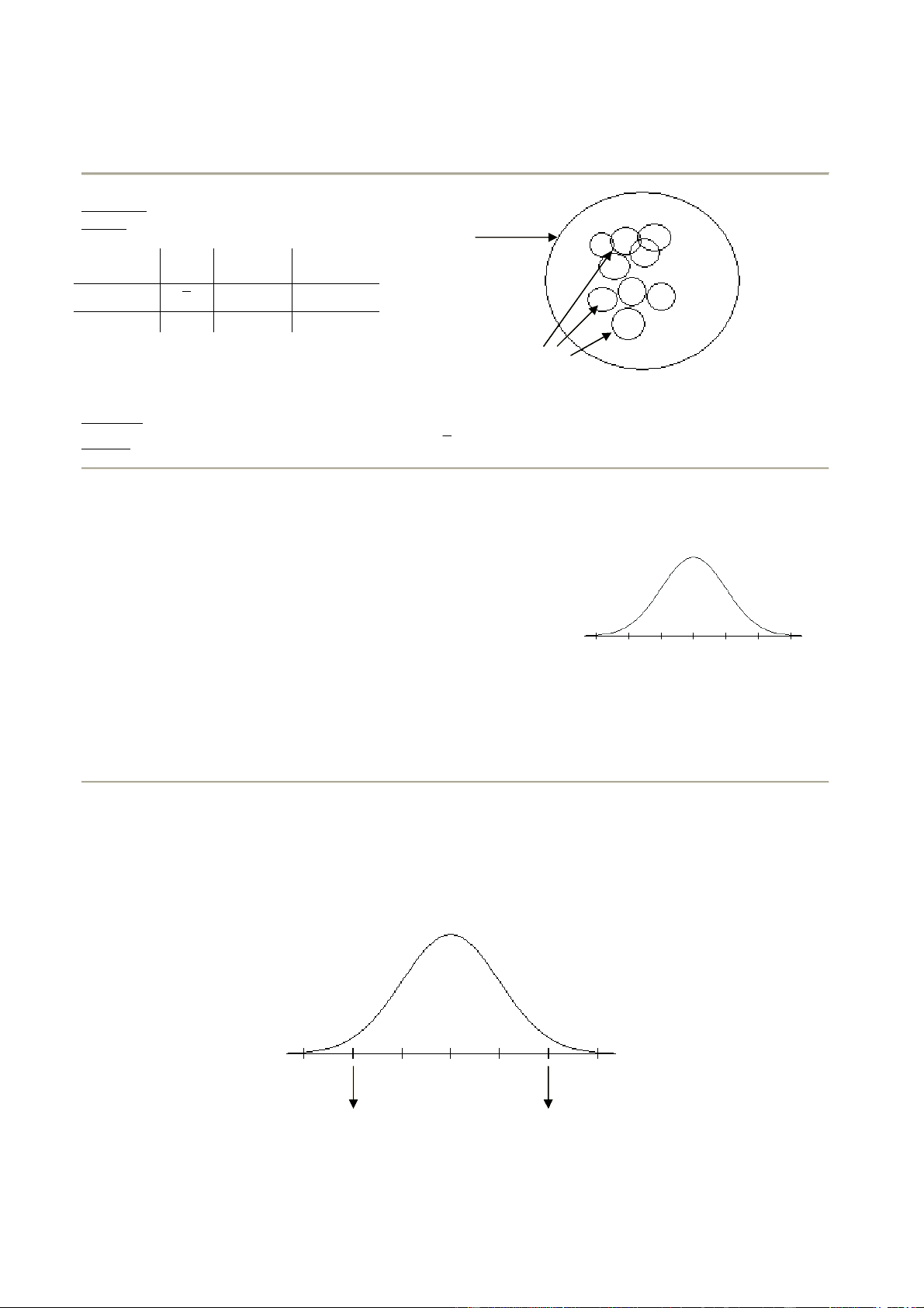
Population: all measurements or observations of interest Sample: a subset of the population population Notation Mean^ StandardDeviation Proportion Sample (^) x S (^) x p ˆ
Population^ μ^ σ p
μ is pronounced “mu” samples σ is pronounced “sigma”
Parameter: a number that describes a population. Examples are μ , σ , and (^) p. Statistic: a number that describes a sample. Examples are x , S (^) x , p ˆ , and n.
A normal curve visually describes a normal distribution. We draw a mathematical model normal curve to represent a normal population distribution. The curve is then used as an approximation to real life normal distributions and is accurate enough for practical purposes. Properties of a normal distribution:
- Is symmetric (so mean = median = center).
- Has one major peak and no outliers.
- Mathematical model (shown to the right) has the x-axis as a horizontal asymptote.
- Area under normal curve equals 1.00. This corresponds to 100% of the data falling below the curve. For a normal distribution the area under a piece of the curve corresponds to the percentage of data along the x-axis under that curve. For example, if the area under a piece of the normal curve is 0.34 then the percentage of data under the curve would be 34%.
If (^) X represents a quantitative variable that is normally distributed then we may write (^) X ~ N (μ , σ). Example: X ~ N ( 17 , 3 )means that the variable X has a normal distribution with mean = μ = 17 and standard deviation = σ = 3.
EMPIRICAL RULE: THE 68-95-99.7 RULE (Applies only to normal distributions!)
- About 68% of the data are within one standard deviation from the mean. In other words, about 68% of the data fall in the interval μ ± 1 σ.
- About 95% of the data are within two standard deviations from the mean. In other words, about 95% of the data fall in the interval μ ± 2 σ.
- About 99.7% of the data are within three standard deviations from the mean. In other words, about 99.7% of the data fall in the interval μ ± 3 σ.
X
μ − 3 σ μ − 1 σ μ μ + 1 σ μ + 3 σ
μ − 2 σ μ + 2 σ
NORMALCDF To calculate the percentage of data under the normal curve between a given lower bound (LB) and upper bound (UB) use normalcdf on your calculator 2 ND^ VARS 2 and enter in the following:
normalcdf (LB, UB, mean of the distribution, standard deviation of the distribution)
If the mean and standard deviation are not entered then the calculator will assume that they are 0 and 1, respectively. Extreme lower bound (like negative infinity) is -1E99 on calculator. Extreme upper bound (like positive infinity) is 1E99 on calculator. To get E on the calculator press 2 ND^ COMMA. The comma button is above the 7 button.
INFO IN PARAGRAPH: WANT TO FIND:
Areaunder thecurvebetweenLBand UB.
Innotation:P(LB X UB)
ProbabilityofchoosingonedatabetweenLBandUB.
ProportionofdatabetweenLBandUB.
Percentageofdata(indecimalform)betweenLBandUB.
LB, UB,mean,standarddeviation Normalcdf
_________________________________________________________________________________
Commute times...
- Assume that commute times of students to school from home are normally distributed with a mean of 17 minutes and a standard deviation of 3 minutes.
a. What percent of students take between 11 and 23 minutes to commute to school? b. What is the probability that a randomly chosen student commutes between 17 and 23 minutes? c. Pat Murphy takes about 20 to 23 minutes to get to school. What is the area under the curve between 20 to 23 minutes? d. What proportion of students take less than 14 minutes to get to school?
IQ scores...
- Suppose that a data set of IQ scores are normally distributed with a mean of 110 and a standard
deviation of 10. In symbols: X ~ N ( 110 , 10 ).
a. What percentage of IQ scores are between 100 and 120? b. What percentage of IQ scores are between 100 and 113? c. What percentage of IQ scores are lower than 95? d. What is the probability of picking an IQ score between 90 and 110? e. Calculate P( 112 < X < 115). f. What is the probability of an IQ score being above 130? g. What proportion of IQ scores are greater than 110? h. What is the area under the normal curve between IQ scores of 103 and 123?
INVNORM To calculate the unknown data X, given the area to the left of X (in decimal form), use Invnorm on your calculator 2 ND^ VARS 3 and enter in the following:
Invnorm (Area to the left, mean of the distribution, standard deviation of the distribution)
If the mean and standard deviation are not entered then the calculator will assume that they are 0 and 1, respectively. Use InvNorm when you are asked to find an unknown number along the horizontal axis that borders a given area.