Galperin-estado solido, Manuais, Projetos, Pesquisas de Física

Baixe Galperin-estado solido e outras Manuais, Projetos, Pesquisas em PDF para Física, somente na Docsity!

Introduction to Modern

Solid State Physics

Yuri M. Galperin

FYS 448

Department of Physics, P.O. Box 1048 Blindern, 0316 Oslo, Room 427A Phone: +47 22 85 64 95, E-mail: iouri.galperinefys.uio.no

• I Basic concepts
• 1 Geometry of Lattices
  • 1.1 Periodicity: Crystal Structures
  • 1.2 The Reciprocal Lattice
  • 1.3 X-Ray Diffraction in Periodic Structures
  • 1.4 Problems
• 2 Lattice Vibrations: Phonons
  • 2.1 Interactions Between Atoms
  • 2.2 Lattice Vibrations
  • 2.3 Quantum Mechanics of Atomic Vibrations
  • 2.4 Phonon Dispersion Measurement
  • 2.5 Problems
• 3 Electrons in a Lattice.
  • 3.1 Electron in a Periodic Field
    • 3.1.1 Electron in a Periodic Potential
  • 3.2 Tight Binding Approximation
  • 3.3 The Model of Near Free Electrons
  • 3.4 Main Properties of Bloch Electrons
    • 3.4.1 Effective Mass
    • 3.4.2 Wannier Theorem → Effective Mass Approach
  • 3.5 Electron Velocity
    • 3.5.1 Electric current in a Bloch State. Concept of Holes.
  • 3.6 Classification of Materials
  • 3.7 Dynamics of Bloch Electrons
    • 3.7.1 Classical Mechanics
    • 3.7.2 Quantum Mechanics of Bloch Electron
  • 3.8 Second Quantization of Bosons and Electrons
  • 3.9 Problems
• II Normal metals and semiconductors ii CONTENTS
• 4 Statistics and Thermodynamics
  • 4.1 Specific Heat of Crystal Lattice
  • 4.2 Statistics of Electrons in Solids
  • 4.3 Specific Heat of the Electron System
  • 4.4 Magnetic Properties of Electron Gas.
  • 4.5 Problems
• 5 Summary of basic concepts
• 6 Classical dc Transport
  • 6.1 The Boltzmann Equation for Electrons
  • 6.2 Conductivity and Thermoelectric Phenomena.
  • 6.3 Energy Transport
  • 6.4 Neutral and Ionized Impurities
  • 6.5 Electron-Electron Scattering
  • 6.6 Scattering by Lattice Vibrations
  • 6.7 Electron-Phonon Interaction in Semiconductors
  • 6.8 Galvano- and Thermomagnetic
  • 6.9 Shubnikov-de Haas effect
  • 6.10 Response to “slow” perturbations
  • 6.11 “Hot” electrons
  • 6.12 Impact ionization
  • 6.13 Few Words About Phonon Kinetics.
  • 6.14 Problems
• 7 Electrodynamics of Metals
  • 7.1 Skin Effect.
  • 7.2 Cyclotron Resonance
  • 7.3 Time and Spatial Dispersion
  • 7.4 Waves in a Magnetic Field
  • 7.5 Problems
• 8 Acoustical Properties...
  • 8.1 Landau Attenuation.
  • 8.2 Geometric Oscillations
  • 8.3 Giant Quantum Oscillations.
  • 8.4 Acoustical properties of semicondictors
  • 8.5 Problems
• 9 Optical Properties of Semiconductors CONTENTS iii
  • 9.1 Preliminary discussion
  • 9.2 Photon-Material Interaction
  • 9.3 Microscopic single-electron theory
  • 9.4 Selection rules
  • 9.5 Intraband Transitions
  • 9.6 Problems
  • 9.7 Excitons
    • 9.7.1 Excitonic states in semiconductors
    • 9.7.2 Excitonic effects in optical properties
    • 9.7.3 Excitonic states in quantum wells
• 10 Doped semiconductors
  • 10.1 Impurity states
  • 10.2 Localization of electronic states
  • 10.3 Impurity band for lightly doped semiconductors.
  • 10.4 AC conductance due to localized states
  • 10.5 Interband light absorption
• III Basics of quantum transport
• 11 Preliminary Concepts
  • 11.1 Two-Dimensional Electron Gas
  • 11.2 Basic Properties
  • 11.3 Degenerate and non-degenerate electron gas
  • 11.4 Relevant length scales
• 12 Ballistic Transport
  • 12.1 Landauer formula
  • 12.2 Application of Landauer formula
  • 12.3 Additional aspects of ballistic transport
  • 12.4 e − e interaction in ballistic systems
• 13 Tunneling and Coulomb blockage
  • 13.1 Tunneling
  • 13.2 Coulomb blockade
• 14 Quantum Hall Effect
  • 14.1 Ordinary Hall effect
  • 14.2 Integer Quantum Hall effect - General Picture
  • 14.3 Edge Channels and Adiabatic Transport
  • 14.4 Fractional Quantum Hall Effect
• IV Superconductivity iv CONTENTS
• 15 Fundamental Properties
  • 15.1 General properties.
• 16 Properties of Type I
  • 16.1 Thermodynamics in a Magnetic Field.
  • 16.2 Penetration Depth
  • 16.3 ...Arbitrary Shape
  • 16.4 The Nature of the Surface Energy.
  • 16.5 Problems
• 17 Magnetic Properties -Type II
  • 17.1 Magnetization Curve for a Long Cylinder
  • 17.2 Microscopic Structure of the Mixed State
  • 17.3 Magnetization curves.
  • 17.4 Non-Equilibrium Properties. Pinning.
  • 17.5 Problems
• 18 Microscopic Theory
  • 18.1 Phonon-Mediated Attraction
  • 18.2 Cooper Pairs
  • 18.3 Energy Spectrum
  • 18.4 Temperature Dependence
  • 18.5 Thermodynamics of a Superconductor
  • 18.6 Electromagnetic Response
  • 18.7 Kinetics of Superconductors
  • 18.8 Problems
• 19 Ginzburg-Landau Theory
  • 19.1 Ginzburg-Landau Equations
  • 19.2 Applications of the GL Theory
  • 19.3 N-S Boundary
• 20 Tunnel Junction. Josephson Effect.
  • 20.1 One-Particle Tunnel Current
  • 20.2 Josephson Effect
  • 20.3 Josephson Effect in a Magnetic Field
  • 20.4 Non-Stationary Josephson Effect
  • 20.5 Wave in Josephson Junctions
  • 20.6 Problems
• 21 Mesoscopic Superconductivity CONTENTS v
  • 21.1 Introduction
  • 21.2 Bogoliubov-de Gennes equation
  • 21.3 N-S interface
  • 21.4 Andreev levels and Josephson effect
  • 21.5 Superconducting nanoparticles
• V Appendices
• 22 Solutions of the Problems
• A Band structure of semiconductors
  • A.1 Symmetry of the band edge states
  • A.2 Modifications in heterostructures.
  • A.3 Impurity states
• B Useful Relations
  • B.1 Trigonometry Relations
  • B.2 Application of the Poisson summation formula
• C Vector and Matrix Relations

vi CONTENTS

Chapter 1

Geometry of Lattices and X-Ray

Diffraction

In this Chapter the general static properties of crystals, as well as possibilities to observe crystal structures, are reviewed. We emphasize basic principles of the crystal structure description. More detailed information can be obtained, e.g., from the books [1, 4, 5].

1.1 Periodicity: Crystal Structures

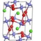
Most of solid materials possess crystalline structure that means spatial periodicity or trans- lation symmetry. All the lattice can be obtained by repetition of a building block called basis. We assume that there are 3 non-coplanar vectors a 1 , a 2 , and a 3 that leave all the properties of the crystal unchanged after the shift as a whole by any of those vectors. As a result, any lattice point R′^ could be obtained from another point R as

R′^ = R + m 1 a 1 + m 2 a 2 + m 3 a 3 (1.1)

where mi are integers. Such a lattice of building blocks is called the Bravais lattice. The crystal structure could be understood by the combination of the propertied of the building block (basis) and of the Bravais lattice. Note that

• There is no unique way to choose ai. We choose a 1 as shortest period of the lattice, a 2 as the shortest period not parallel to a 1 , a 3 as the shortest period not coplanar to a 1 and a 2.
• Vectors ai chosen in such a way are called primitive.
• The volume cell enclosed by the primitive vectors is called the primitive unit cell.
• The volume of the primitive cell is V 0

V 0 = (a 1 [a 2 a 3 ]) (1.2)

1.1. PERIODICITY: CRYSTAL STRUCTURES 5

White and black circles are the atoms of different kind. a is a primitive lattice with one atom in a primitive cell; b and c are composite lattice with two atoms in a cell.

Two-Dimensional Lattices

The are 5 basic classes of 2D lattices (see Fig. 1.3)

Figure 1.3: The five classes of 2D lattices (from the book [4]).

6 CHAPTER 1. GEOMETRY OF LATTICES ...

Three-Dimensional Lattices

There are 14 types of lattices in 3 dimensions. Several primitive cells is shown in Fig. 1.4. The types of lattices differ by the relations between the lengths ai and the angles αi.

Figure 1.4: Types of 3D lattices

We will concentrate on cubic lattices which are very important for many materials.

Cubic and Hexagonal Lattices. Some primitive lattices are shown in Fig. 1.5. a, b, end c show cubic lattices. a is the simple cubic lattice (1 atom per primitive cell), b is the body centered cubic lattice (1/ 8 × 8 + 1 = 2 atoms), c is face-centered lattice (1/ 8 × 8 + 1/ 2 × 6 = 4 atoms). The part c of the Fig. 1.5 shows hexagonal cell.

8 CHAPTER 1. GEOMETRY OF LATTICES ...

Figure 1.7: More symmetric choice of lattice vectors for bcc lattice.

The procedure is outlined in Fig. 1.8. For complex lattices such a procedure should be done for one of simple sublattices. We shall come back to this procedure later analyzing electron band structure.

Figure 1.8: To the determination of Wigner-Seitz cell.

1.2 The Reciprocal Lattice

The crystal periodicity leads to many important consequences. Namely, all the properties, say electrostatic potential V , are periodic

V (r) = V (r + an), an ≡ n 1 a 1 + n 2 a 2 + n 2 a 3. (1.3)

1.2. THE RECIPROCAL LATTICE 9

It implies the Fourier transform. Usually the oblique co-ordinate system is introduced, the axes being directed along ai. If we denote co-ordinates as ξs having periods as we get

V (r) =

∑^ ∞

k 1 ,k 2 ,k 3 =−∞

Vk 1 ,k 2 ,k 3 exp

[

2 πi

s

ksξs as

]

Then we can return to Cartesian co-ordinates by the transform

ξi =

k

αikxk (1.5)

Finally we get V (r) =

b

Vbeibr^. (1.6)

From the condition of periodicity (1.3) we get

V (r + an) =

b

Vbeibreiban^. (1.7)

We see that eiban^ should be equal to 1, that could be met at

ba 1 = 2πg 1 , ba 2 = 2πg 2 , ba 3 = 2πg 3 (1.8)

where gi are integers. It could be shown (see Problem 1.4) that

bg ≡ b = g 1 b 1 + g 2 b 2 + g 3 b 3 (1.9)

where

b 1 =

2 π[a 2 a 3 ] V 0 , b 2 =

2 π[a 3 a 1 ] V 0 , b 3 =

2 π[a 1 a 2 ] V 0

It is easy to show that scalar products

aibk = 2πδi,k. (1.11)

Vectors bk are called the basic vectors of the reciprocal lattice. Consequently, one can con- struct reciprocal lattice using those vectors, the elementary cell volume being (b 1 [b 2 , b 3 ]) = (2π)^3 /V 0.

Reciprocal Lattices for Cubic Lattices. Simple cubic lattice (sc) has simple cubic reciprocal lattice with the vectors’ lengths bi = 2π/ai. Now we demonstrate the general procedure using as examples body centered (bcc) and face centered (fcc) cubic lattices. First we write lattice vectors for bcc as a 1 = a 2

(y + z − x) ,

a 2 = a 2 (z + x − y) ,

a 1 = a 2 (x + y − z) (1.12)

1.3. X-RAY DIFFRACTION IN PERIODIC STRUCTURES 11

which acts upon a periodic structure. Each atom placed at the point ρ produces a scattered spherical wave

Fsc(r) = f F(ρ) eikr r = f F 0 eikρei(kr−ωt) r

where r = R − ρ cos(ρ, R), R being the detector’s position (see Fig. 1.10) Then, we

Figure 1.10: Geometry of scattering by a periodic atomic structure.

assume R  ρ and consequently r ≈ R; we replace r by R in the denominator of Eq. (1.15). Unfortunately, the phase needs more exact treatment:

kρ + kr = kρ + kR − kρ cos(ρ, R). (1.16)

Now we can replace kρ cos(ρ, R) by k′ρ where k′^ is the scattered vector in the direction of R. Finally, the phase equal to

kR − ρ∆k, ∆k = k − k′.

Now we can sum the contributions of all the atoms

Fsc(R) =

m,n,p

fm,n,p

F 0

ei(kR−ωt) R

) [

exp(−iρm,n,p∆k

]

If all the scattering factors fm,n,p are equal the only phase factors are important, and strong diffraction takes place at ρm,n,p∆k = 2πn (1.18)

with integer n. The condition (1.18) is just the same as the definition of the reciprocal vectors. So, scattering is strong if the transferred momentum proportional to the reciprocal lattice factor. Note that the Laue condition (1.18) is just the same as the famous Bragg condition of strong light scattering by periodic gratings.

12 CHAPTER 1. GEOMETRY OF LATTICES ...

Role of Disorder

The scattering intensity is proportional to the amplitude squared. For G = ∆k where G is the reciprocal lattice vector we get

Isc ∝ |

i

eiGRi^ | · |

i

e−iGRi^ | (1.19)

or Isc ∝ |

i

i

j 6 =i

eiG(Ri−Rj^ )|. (1.20)

The first term is equal to the total number of sites N , while the second includes correlation. If G(Ri − Rj ) ≡ GRij = 2πn (1.21)

the second term is N (N − 1) ≈ N 2 , and

Isc ∝ N 2.

If the arrangement is random all the phases cancel and the second term cancels. In this case Isc ∝ N

and it is angular independent. Let us discuss the role of a weak disorder where Ri = R^0 i + ∆Ri

where ∆Ri is small time-independent variation. Let us also introduce

∆Rij = ∆Ri − ∆Rj.

In the vicinity of the diffraction maximum we can also write

G = G^0 + ∆G.

Using (1.20) and neglecting the terms ∝ N we get

Isc(G 0 + ∆G) Isc(G 0 )

i,j exp^

[

i

G^0 ∆Rij + ∆GR^0 ij + ∆G∆Rij

)]

i,j exp [iG^0 ∆Rij^ ]^

So we see that there is a finite width of the scattering pattern which is called rocking curve, the width being the characteristics of the amount of disorder. Another source of disorder is a finite size of the sample (important for small semicon- ductor samples). To get an impression let us consider a chain of N atoms separated by a distance a. We get

|

N∑ − 1

n=

exp(ina∆k)|^2 ∝ sin^2 (N a∆k/2) sin^2 (a∆k/2)

This function has maxima at a∆k = 2mπ equal to N 2 (l‘Hopital’s rule) the width being ∆k′a = 2. 76 /N (see Problem 1.6).